In this post, I will provide links to standard benchmark datasets that can be used for frequent subgraph mining. Moreover, I will provide a set of small graph datasets that can be used for debugging subgraph mining algorithms.
The format of graph datasets
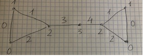
A graph dataset is a text file which contains one or more graphs. A graph is defined by a few lines of text that follow the following format (used by the GSpan algorithm)
t # N This is the first line of a graph. It indicates that this is the N-th graph in the file
v M L This line defines the M-th vertex of the current graph, which has a label L
e P Q L This line defines an edge, which connects the P-th vertex with the Q-th vertex. This edge has the label L
Small datasets for debugging
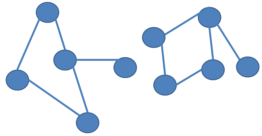
Here are some small datasets that can be used for debugging frequent subgraph mining algorithms. Each dataset contains one or two graphs, which is enough for some small debugging tasks.
In this blog post, I have share some helpful datasets. If you want to know more about subgraph mining you may read my short introduction to subgraph mining.
— Philippe Fournier-Viger is a professor of Computer Science and also the founder of the open-source data mining software SPMF, offering more than 145 data mining algorithms.
In this blog post, I will briefly discuss the fact that the popular CloSpan algorithm for frequent sequential pattern mining is an incomplete algorithm. This means that in some special situations, CloSpan does not produce the expected results that it has been designed for, and in particular some patterns are missing from the final result. I will try to give a brief explanation of that problem but I will refer to another paper for the actual proof that the algorithm is incomplete. Moreover, I will briefly talk about a similar problem in the IncSpan algorithm.
What is CloSpan?
CloSpan is one of the most famous algorithm for sequential pattern mining. It is designed for discovering subsequences that appear frequently in a set of sequence. CloSpan was published in 2003 in the famous SIAM Data Mining conference:
[1] Yan, X., Han, J., & Afshar, R. (2003, May). CloSpan: Mining: Closed sequential patterns in large datasets. In Proceedings of the 2003 SIAM international conference on data mining (pp. 166-177). Society for Industrial and Applied Mathematics.
The SIAM DM conference is a top conference. And the CloSpan paper has been cited in more than 940 papers, and used by many researchers.
What is CloSpan used for?
The CloSpan algorithm takes as input a parameter called minsup and a sequence database (a set of sequences). A sequence is an ordered list of itemsets. An itemset is a set of symbols. For example, consider the following sequence database, which contains three sequences:
Here the first sequence (Sequence 1) means that a customer has bought the items bread and apple together, has then bought milk and apple together, and then has bought bread. Thus, this sequence contains three itemsets. The first itemset is bread with apple. The second itemset is milk with apple. The third itemset is bread.
In sequential pattern mining the goal is to find all subsequences that appears in at least minsup sequences of a database (all the sequential patterns). For example, consider the above database and that minsup = 2 sequences. Then, subsequence <(bread, apple),(apple)(bread)> is a sequential pattern since it appears in two sequences of the above database, which is no less than minsup. A sequential pattern mining algorithm should be able to find all subsequences that meet this criterion, that is to find all sequential patterns. Above I have given a quite informal definition with an example. If you want more details about this problem, you could read my survey paper about sequential pattern mining, which gives a more detailed overview of this problem.
The CloSpan algorithm is an algorithm to find a special type of sequential patterns called the closed sequential patterns (see the above survey for more details).
What is the problem?
In algorithmic two important aspects are often discussed when talking about some algorithms. They are whether an algorithm is correct or incorrect, and whether it is complete or incomplete. For the problem of sequential pattern mining, a complete algorithm is an algorithm that can find all the required sequential patterns, and a correct algorithm is one that will correctly calculate the number of occurrences of each pattern found (correctly calculate the support).
Now the problem with CloSpan is that it an incomplete algorithm. It applies some theoretical results (Theorem 1, Lemma 3 and Corollary 1-2 in [1]) to reduce the search space, which work well for some databases containing only sequences of itemsets containing a single item each. But in some cases where a database contains sequences of itemsets containing more than one item per itemset, the algorithm can miss some sequential patterns. In other words, the CloSpan algorithm is incomplete. In particular, in the following paper [2], it was shown that the Theorem 1, Lemma 3 and Corollary 1-2 of the original CloSpan paper are incorrect.
[2] Le, B., Duong, H., Truong, T., & Fournier-Viger, P. (2017). FCloSM, FGenSM: two efficient algorithms for mining frequent closed and generator sequences using the local pruning strategy. Knowledge and Information Systems, 53(1), 71-107.
In [2], this was shown with an example (Example 2) and it was also shown experimentally that if the original Corollary 1 of CloSpan is used, patterns can be missed. For example, on a dataset called D0.1C8.9T4.1N0.007S6I4, CloSpan can find 145,319 patterns, while other algorithms for closed sequential pattern mining can find 145,325 patterns. Thus, patterns can be missed, although not necessarily many.
I will not discussed the details about why the results are incomplete as it would requires too much explanations for a blog post. But for those interested, you can check the above paper [2] which has clearly explained the problem.
And what about other algorithms?
In this blog post, I have discussed a theoretical problem in the CloSpan algorithm such that CloSpan is incomplete in some cases. This result was presented in the paper [2]. But to ensure more visibility for this result, as CloSpan is a popular algorithm, I thought that it would be a good idea to write a blog post about this result.
By the way, this is not the only sequential pattern mining algorithm that is incorrect or incomplete. Another famous sequential pattern mining that is incorrect is IncSpan for incremental sequential pattern mining, published in the KDD 2004 conference, and cited in more than 240 papers:
[3] Cheng, H., Yan, X., & Han, J. (2004, August). IncSpan: incremental mining of sequential patterns in large database. In Proceedings of the tenth ACM SIGKDD international conference on Knowledge discovery and data mining (pp. 527-532). ACM.
After the paper about IncSpan was published, the following year, it was shown in a PAKDD paper[4] that IncSpan is incomplete (it can miss some patterns). In that same paper, a complete algorithm called IncSpan+ was proposed. This is the paper [4] that has demonstrated that IncSpan is incomplete:
Nguyen, S. N., Sun, X., & Orlowska, M. E. (2005, May). Improvements of IncSpan: Incremental mining of sequential patterns in large database. In Pacific-Asia Conference on Knowledge Discovery and Data Mining (pp. 442-451). Springer, Berlin, Heidelberg.
Conclusion
The lesson to learn from this is that it is important to check the correctness and completeness of algorithms carefully before publishing a paper. And it also highlights that errors can also be found even in papers published in the very top conferences of the field, as reviewers often do not have time to check all the details of a paper, and papers sometimes do not include a detailed proof that algorithms are correct and complete. But although I have highlighted two cases with CloSpan and IncSpan, there are not the only papers to have theoretical problems. It happens quite often, actually.
== Philippe Fournier-Viger is a full professor and the founder of the open-source data mining software SPMF, offering more than 110 data mining algorithms. If you like this blog, you can tweet about it and/or subscribe to my twitter account @philfv to get notified about new posts.
Today, I will discuss 10 ways of becoming more efficient at doing research. This is an important topic for any researcher who wishes to be more productive in terms of research. For example, one may want to be able to publish more research papers and be involved in more projects without decreasing the overall quality of the papers/projects.
So how to be more efficient? Here is my advice:
Prioritize your tasks. Since there are only 24 hours in a day, to be more efficient, it is important to better manage the time to do what is the most important first.
Select your tasks. Moreover, one choose to do tasks that provide the greatest reward and not do what is unimportant and provide a small reward. Thus, it is better to wisely choose the research projects that are the most promising and require less time to complete, or that require more time but can provide a greater reward (such as publishing in a top journal). Besides, when doing a research project, it is important to think about the benefit that each hour/day of work will provide as a reward. For example, if you are designing a software but have to work one week to add a feature, then you should ask yourself if adding that feature is worth that time or if adding some other alternative features will provide a greater reward. If the feature is not really important, then you should perhaps not add the feature and focus on something else that is more important to improve your research project.
Ask other people to participate to your projects. If one works by himself, he will be limited by his time and ability. But if one invites other researchers to their project, he can delegate tasks to other people such as writing, programming and carrying experiments. Thus, the project may be completed faster and the quality may also be improved by having the opinion and using the special skills of other people.
Participate to other people’s projects. It is also important to participate to the projects of other researchers. This helps to increase the global number of papers and projects that one can do and open also other opportunities (recommendation letter, invitation to give a talk, invitation to participate in a committee, etc.).
Write down your ideas. Many people have difficulty to find ideas for research projects. However, everybody has ideas everyday but often forget them because they don’t take notes. The solution is to take notes in a file or notebook every time that you have an idea. I personally do this all the time. For example, if I read some papers and think about some opportunity for a new project, I will write it down in my notebook of ideas. Then, when it is time to start a new project, I will look at my list of ideas and choose something as the basis for a new project. This greatly helps to find good new research topics.
Having a healthy lifestyle. This is quite obvious but many people do not pay attention to this. It is important to eat well, do exercise, as well as sleeping enough and having a regular schedule. It is easy to think that sleeping less is useful but in the end there is never any benefit to doing this as the body will need to sleep more the following day, and being tired the following day will decrease the productivity. Thus, it is better to manage the time properly to finish projects before deadlines and avoid sleeping very late to finish projects.
Avoid sources of distractions and work in a suitable location. It is often tempting to do something else while working such as listening to music or watching TV, or to work in a non optimal environment such as working while laying in the bed or on the couch. However, this can greatly decrease productivity and in some case barely any work is done. For example, I can rarely work well while listening to music except when doing some repetitive tasks or sometimes when programming. Another source of distraction may be instant messages and other forms of events that can interrupt your work. Also, it is useful to keep the workplace clean and ordered to help you focus on your task.
Take some breaks. After working for a long time, it is good to take a break, go for a walk, and then come back to work later more efficiently. Moreover, one can take advantage of the breaks to focus on the distractions such as taking phone calls and answering instant messages that were ignored when working. For example, it is a good habit to go for a short walk after working for a 1 or 2 hours. And during that time, it is possible to think about the problem to be solved or just have a rest. Sometimes thinking about a problem without being in front of the computer (e.g. while walking) can bring some new ideas.
Keep meeting short and focused. It is tempting to do meetings every week or to have very long meetings. In my opinion, it is better to do the meetings only when necessary and to keep them focused on what is really important, and take notes. Meetings can consume a lot of time.
Set some goals and rewards. Another way of increasing efficiency is to set some clear goals and deadlines to put pressure on yourself to finish these tasks on time. Moreover, you can also set some rewards that you will give to yourself after completing a task. For example, one can say that after finishing a certain task at a given deadline, he may go to see a movie as a reward.
Conclusion
In this blog post, I have discussed several ways of increasing research efficiency that are simple but really works! 🙂
Hope that you have enjoyed this blog post. If so, there are many other topics on this blog that you may be interested in! So please keep reading 🙂 Also, please leave comments below if you have other suggestions or want to share your experience about how to do research efficiently.
== Philippe Fournier-Viger is a full professor and the founder of the open-source data mining software SPMF, offering more than 110 data mining algorithms. If you like this blog, you can tweet about it and/or subscribe to my twitter account @philfv to get notified about new posts.
In this blog post, I will explain why the FSMS algorithm for frequent subgraph mining is an incorrect algorithm. I will publish this blog post because I have found that the algorithm is incorrect after spending a few days to implement the algorithm in 2017 and wish to save time to other researchers who may also want to implement this algorithm.
This post will assume that the reader is familiar with the FSMS algorithm, published in the proceedings of the Industrial Conference on Data Mining.
Abedijaberi A, Leopold J. (2016) FSMS: A Frequent Subgraph Mining Algorithm Using Mapping Set, Proceedings of the 16th Industrial Conference on Data Mining (Ind. CDM 2016). Springer, 2016: 761-773.
I will first give a short summary of why the algorithm is incorrect and then give a detailled example to illustrate the problem.
Brief summary of the problem
The FSMS algorithm creates some mapping sets. The purpose of a mapping set is to keep track of vertices that are isomorphic for different subgraph instances. But I have found that in some cases we can expand a subgraph instance from two different vertices that are not isomorphic according to the mapping set but that will still generate some graph instances that are isomorphic. The problem that occurs is that FSMS does not detect that these graph instances are isomorphic using the mapping sets.
Thus, the support of subgraphs may be incorrectly calculated and some frequent subgraphs may be missing from the output of the algorithm.
Example
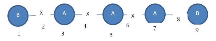
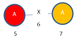
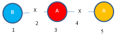
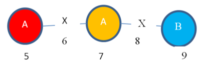
The above short description may not be clear. So let me explain this now with an example. Consider that we have the following graph with five vertices and two edges. The vertex labels are A, B and the edge label is X. The numbers 1,2,3,4,5…9 are some ids that I will use for the purpose of explanation.
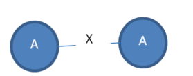
In the above graph, I can find various subgraphs. Consider the following subgraph that I will call “Subgraph1”:
Subgraph1:
The subgraph “Subgraph1” has two instances:
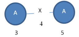
Instance 1:
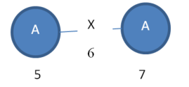
Instance 2:
Moreover, we can say that “Subgraph 1” has a support of 2.
We can also say that “Subgraph 1” has the following values: VALUES 3-4-5 VALUES 5-6-7 and the following mapping set: A = 3,5 A = 5,7
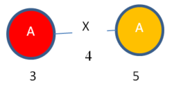
Just to make my example easier to understand, we can visualize these mapping set entries of “Subgraph 1” using colors. We have two entries. One is RED. The other one is ORANGE.
Instance 1:
Instance 2:
Ok, so we have a subgraph called “Subgraph 1” and we have its mapping set. Now, let’s continue my example. We will expand our subgraph “Subgraph 1” to find larger subgraph(s). According to the FSMSalgorithm, we should find the edges that extend each mapping set entry (each color), as we know that this will generate some subgraphs that are isomorphic.
So, I can expand vertex 3 of “Instance 1” to obtain this subgraph instance:
Instance 4:
Moreover, I can expand vertex 7 of “Instance 2” to obtain this subgraph instance:
Instance 5:
Obviously, “Instance 4” and “Instance 5” are isomorphic.
But the problem that I have found is that these two instances are not obtained by expanding the same entries in the mapping sets of “Subgraph 1”. To obtain “Instance 4” I have expanded the RED entry of the mapping set (vertex 3). But to obtain “Instance 5”, I have expanded the ORANGE entry of the mapping set (vertex 7). But the resulting instances (“Instance 4” and “Instance 5”) are isomorphic.
Thus the FSMS algorithm is unable to detect that these two instances (“Instance 4” and “Instance 5”) are isomorphic.
If these two instances had been obtained by expanding vertices from the same mapping set entry (color) of “Subgraph1”, we would know that “Instance 4” and “Instance 5” are isomorphic. But in my example, these two instances are not obtained by extending the same entry of the mapping set of “Subgraph 1”.
When this problem occurs?
My above example is very simple. But the same problem can happen for larger subgraphs with more edges. In general, how can we detect that extending different entries (colors) of a mapping set yield isomorphic graph instances? Actually, this problem only occurs if we have many nodes with the same label. If we do not have many nodes with the same labels, it will not happen. But we still need to deal with this problem since in real-life a graph may have multiple vertices with the same labels.
Can this problem be fixed?
There does not seem to be a simple solution to fix the problem. Actually, one may think that a solution is to perform isomorphic tests. But the FSMSalgorithm was designed to avoid isomorphic tests. Thus, it would defeat the purpose of the algorithm. I have thought about it for a while but did not find any simple solution to fix the algorithm.
Conclusion
In this blog post, I have reported a problem in the FSMSalgorithm such that the resultis incorrect. I have actually implemented the algorithm and tested it extensively, which has led to finding this issue. If someone is interested in obtaining the Java implementation of the algorithm that I have made, I could share it by e-mail.
The other conclusion that can be made is that it is easy to overlook some cases when designing and algorithm. There are actually several published algorithms that contain errors, even in top conferences/journals. For researchers, a solution to avoid such issue is to always provide a proof of correctedness/completedness, and to extensively test an implementation for bugs.
== Philippe Fournier-Viger is a full professor and the founder of the open-source data mining software SPMF, offering more than 110 data mining algorithms. If you like this blog, you can tweet about it and/or subscribe to my twitter account @philfv to get notified about new posts.
Many researchers are not native English speakers but need to write research papers in English, as it is the common language for sharing ideas with other researchers worldwide. Some papers are very well-written, others are not so well-written but are still readable, while others are hard to read and really need to be improved. In recent years, more and more publishers have thus started to offer manuscript proofreading services to authors. In theory, this sounds like a good idea since it can help to improve the papers of authors and ensure that all papers are well-written before they are published. However, in this blog post, I will highlight that there is a potential conflict of interest as some of these proofreading services are aggresively pushed by publishers, and can be an important revenue stream for publishers. In particular, I will discuss the case of the IEEE.
Recently, a friend of mine submitted a manuscript to an IEEE journal. After waiting a few weeks, he received the following e-mail:Date: (…) 2018 Dear Dr. Z.X.We are writing to you in regards to Manuscript ID XXXXXX entitled “XXXXXX” which you submitted to IEEE XXXX.Your paper was read with interest, however; the grammar needs improvement. Proper grammar is a requirement for publication in IEEE XXXX. If needed, IEEE offers a 3rd party service for language polishing, for a fee: https://www.aje.com/c/ieee (use the URL to claim a 10% discount).
Your article has been returned to your Author Center so that you can resubmit after you have improved the grammar. You will be unable to make your revisions on the originally submitted version of your manuscript. Instead, revise your manuscript using a word processing program and save it on your computer.(…)IEEE XXXX Editorial Office
It is interesting to note that this e-mail sent by the IEEE editorial office states that the “paper was read with interest” but that e-mail does not include any reviews from reviewers. Thus, it seems that the paper was not reviewed and just returned directly to authors. Besides, it is interesting that this e-mail is sent by “the IEEE XXX Editorial office” and is not signed by an editor. If the paper was not well-written, it would make sense to suggest to improve the English so that it reaches a satisfactory level. However, I have actually checked the paper and the English is OK. It is not perfect since the author is not a native speaker. Indeed, there was a few sentences in that paper that did not sound totally right in English and a few typos. But the paper was on overall readable and in my opinion acceptable in terms of English. Thus, this raises questions about the reason for suggesting that the language should still be polished. In particular, it seems that the IEEE is even refusing to send the paper to reviewers although the paper is in my opinion readable at a reasonable level.
If the IEEE affiliated language polishing service was not mentionned in the e-mail, there would not be a potential conflict of interest. But in that e-mail, it seems like the IEEE is trying to push authors to use their services and suggest to authors that otherwise the paper will not even be submitted to reviewers, which put a huge amount of pressure on authors to use the recommended language polishing service or others.
If this an isolated case? Actually, I have asked some of my colleagues, and they also received a similar e-mail from the IEEE a few months ago when submitting their paper to the same journal. I did not check the paper but here is the e-mail:
Date: Thu, Nov 30, 2017 at 6:59 AM Subject: IEEE XXXXXx- Instructions to Resubmit Manuscript
Dear Prof. XXXXX
We are writing to you in regards to XXXXX which you submitted to IEEE XXXXX.
Your paper was read with interest, however; the grammar needs improvement. Proper grammar is a requirement for publication in IEEE XXXXX. If needed, IEEE offers a 3rd party service for language polishing, for a fee: https://www.aje.com/c/ieee (use the URL to claim a 10% discount).
Your article has been returned to your Author Center so that you can resubmit after you have improved the grammar. (…)
The e-mail also did not contain reviews.
Is this only the IEEE? There are other publishers who are affiliated to language proofreading services. For example, on the website of Springer, one can see that they offer a similar service. However, by looking at the acceptance notification of papers in Springer journals received by me and my colleagues, I did not see them pushing their language services as aggressively as the IEEE in the two above examples.
Besides, in the above e-mails, the IEEE is not disclosing whether they receive money for promoting the “third party” language editing service. But it seems likely. Otherwise, why would they do it?
Conclusion
In this blog post, I have discussed a potential conflict of interest between the fact that some publishers like IEEE are pushing affiliated language proofreading services and likely earning money from it. I have discussed two cases related to some IEEE journal. However, it may be different for other journals and publishers. If someone has additional interesting information related to this topic, either for the IEEE or other publishers, please share in the comments below of by e-mail, and I will update the blog post.
== Philippe Fournier-Viger is a full professor and the founder of the open-source data mining software SPMF, offering more than 110 data mining algorithms. If you like this blog, you can tweet about it and/or subscribe to my twitter account @philfv to get notified about new posts.
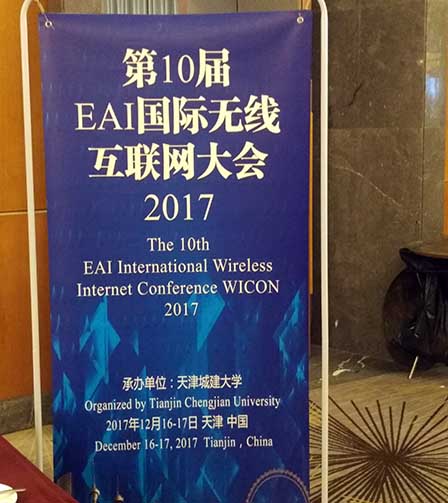
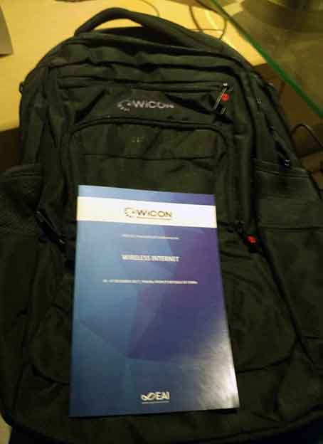
This week-end, I have attended the WICON 2017 conference in Tianjin, China to present a research paper about the application of data mining to analyze data from water meters installed in the City of Moncton, Canada. In this post, I will give a brief overview of the WICON 2017 conference.
About the conference
This was the 10th edition of theWICONconference (International Conference on Wireless Internet), which is organized by the EAI (European Alliance for Innovation). The conference is about networking and is attended by both researchers from computer sciences and engineering. This year, the conference was held at the Holiday Inn hotel in Tianjin, China which is a major Chinese city having historical importance.
Tianjin, China
The conference was held in a room on the fifth floor of the hotel. There seemed to be 30 to 40 attendees at the conference opening:
The conference opening
Conference proceedings
The conference proceedings are published by Springer, which ensures some visibility and that paper will be indexed in various publication databases. However, at the time of attending the conference, the proceedings were not available on USB or as a book. Only a download link was provided the day before the conference to the attendees. It was said that the reason for not providing a USB or book is that the conference proceedings will be published after the conference. Each attendee receive a conference bag and a booklet indicating the conference program.
Acceptance rate
About the acceptance rate, it was announced that 85 papers were received from 10 countries. From those, 15 were rejected before the review process. And then, 43 papers were accepted. Thus, the acceptance rate is 62%.
The conference is an international conference. But the majority of the papers were from China. In the program there is about 2 papers with a majority of authors from Canada, 1 from Morroco and 1 from Senegal.
The program committee of the conference is quite international though, and the conference has been held in various countries including United states, Hungary, and Portugal. But in recent years, this conference seems to have been more focused on China as four of the last five editions were in China.
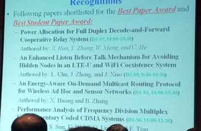
Best paper award
Four papers were nominated for the best paper award.
It was announced in the conference booklet that the best paper award would be announced at the conference gala/dinner held in the evening of the first day. But it was actually announced on the morning of the second day. I did not note take note of who the winners were.
Conference gala/dinner
According to the booklet, a conference gala/dinner was to be held from 19:00 to 22:00. However, on the ticket, it was written 18:00 to 20:30. This actually created some confusion. I asked some people at 17:50 (at the end of the technical session) and they told me to go to the hotel restaurant at 18:00. Thus, I was there from 18:00 to 19:20 and I just sat at a table eating while a few people from the conferences were eating at other tables. Then, at 19:00, a few more people from the conference started to arrive (those who thought there would be a gala at 19:00). But there was actually no announcements or gala (at least during the time that I was sitting there), so I finally went back to work in my hotel room after a while.
Topics of the conference
The conference is about networks. It had various tracks. The papers were about topics such as: clustering for spectrum resource allocation, clustering applied to monitor wireless sensor networks, evaluation of multi-channel CSMA, MIMO and mmWave, Vehicular networks (VANETS), routing protocols, security and internet of things, swarm of drones for intrusion detection, analysis of mobile traffic, networking algorithms and protocols, and cloud and big data networking using fuzzy logic, haze prediction and clustering.
There was two keynotes by some good researchers in the field of networking. One of them was about his research on applying deep learning for routing traffic, which is an interesting approach. That approach appeared to give good results. However, there remain some challenges as examples were given with a small network (about 16 nodes), and it was said that the computing cost is very high (something that could maybe useful in 20 to 30 years from now). For the first keynote, I try to recall the title, but cannot find the title or abstract in the conference booklet or website.
Conclusion
It was on overall interesting to attend this conference, although I must say that this conference is a little bit outside my field (I usually attend artificial intelligence and data mining conferences). The conference is not very big, so the opportunities for networking are limited compared to larger conferences. A good point is that this conference is published by Springer.
== Philippe Fournier-Viger is a full professor and the founder of the open-source data mining software SPMF, offering more than 110 data mining algorithms. If you like this blog, you can tweet about it and/or subscribe to my twitter account @philfv to get notified about new posts.
This blog post provides an introduction to the Apriori algorithm, a classic data mining algorithm for the problem of frequent itemset mining. Although Apriori was introduced in 1993, more than 20 years ago, Apriori remains one of the most important data mining algorithms, not because it is the fastest, but because it has influenced the development of many other algorithms.
The problem of frequent itemset mining
The Apriorialgorithm is designed to solve the problem of frequent itemset mining. I will first explain this problem with an example. Consider a retail store selling some products. To keep the example simple, we will consider that the retail store is only selling five types of products: I= {pasta, lemon, bread, orange, cake}. We will call these products “items”.
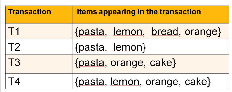
Now, assume that the retail store has a database of customer transactions:
This database contains four transactions. Each transaction is a set of items purchased by a customer (an itemset). For example, the first transaction contains the items pasta, lemon, bread and orange, while the second transaction contains the items pasta and lemon. Moreover, note that each transaction has a name called its transaction identifier. For example, the transaction identifiers of the four transactions depicted above are T1, T2, T3 and T4, respectively.
The problem offrequent itemset mining is defined as follows. To discover frequent itemsets, the user must provide a transaction database (as in this example) and must set a parameter called the minimum support threshold (abbreviated as minsup). This parameter represents the number of transactions that an itemset should at least appear in to be considered a frequent itemset and be shown to the user. I will explain this with a simple example.
Let’s say that the user sets the minsup parameter to two transactions (minsup = 2 ). This means that the user wants to find all sets of items that are purchased together in at least two transactions. Those sets of items are called frequent itemsets. Thus, for the above transaction database, the answer to this problem is the following set of frequent itemsets:
All these itemsets are considered to be frequent itemsets because they appear in at least two transactions from the transaction database.
Now let’s be a little bit more formal. How many times an itemset is bought is called the support of the itemset. For example, the support of {pasta, lemon} is said to be 3 since it is appears in three transactions. Note that the support can also be expressed as a percentage. For example, the support of {pasta, lemon} could be said to be 75% since pasta and lemon appear together in 3 out of 4 transactions (75 % percent of the transactions in the database).
Formally, when the support is expressed as a percentage, it is called a relative support, and when it is expressed as a number of transactions, it is called an absolute support.
Thus, the goal of frequent itemset mining is to find the sets of items that are frequently purchased in a customer transaction database (the frequent itemsets).
Applications of frequent itemset mining
Frequent itemset mining is an interesting problem because it has applications in many domains. Although, the example of a retail store is used in this blog post, itemset mining is not restricted to analyzing customer transaction databases. It can be applied to all kind of data from biological data to text data. The concept of transactions is quite general and can be viewed simply as a set of symbols. For example, if we want to apply frequent itemset mining to text documents, we could consider each word as an item, and each sentence as a transaction. A transaction database would then be a set of sentences from a text, and a frequent itemset would be a set of words appearing in many sentences.
The problem of frequent itemset mining is difficult
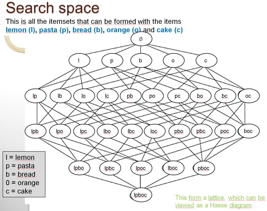
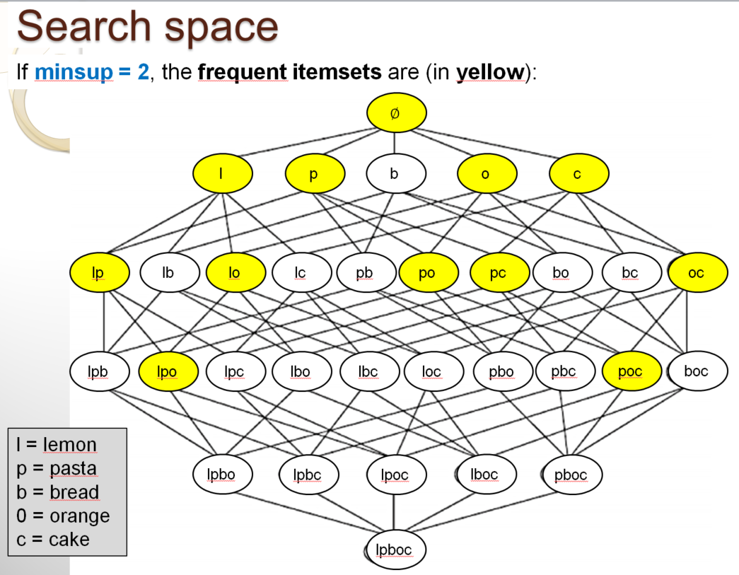
Another reason why the problem of frequent itemset mining is interesting is that it is a difficult problem. The naive approach to solve the problem of itemset mining is to count the support of all possible itemsets and then output those that are frequent. This can be done easily for a small database as in the above example. In the above example, we only consider five items (pasta, lemon, bread, orange, cake). For five items, there are 32 possible itemsets. I will show this with a picture:
In the above picture, you can see all the sets of items that can be formed by using the five items from the example. These itemsets are represented as a Hasse diagram. Among all these itemsets, the following itemsets highlighted in yellow are the frequent itemsets:
Now, a good question is: how can we write a computer program to quickly find the frequent itemsets in a database? In the example, there are only 32 possible itemsets. Thus, a simple approach is to write a program that calculate the support of each itemset by scanning the database. Then, the program would output the itemsets having a support no less than the minsup threshold to the user as the frequent itemsets. This would work but it would be highly inefficient for large databases. The reason is the following.
In general, if a transaction database has x items, there will be 2^x possible itemsets (2 to the power of x). For example, in our case, if we have 5 items, there are 2^5 = 32 possible itemsets. This is not a lot because the database is small. But consider a retail store having 1,000 items. Then the number of possible itemsets would be: 2^1000 = 1.26 E30, which is huge, and it would simply not be possible to use a naive approach to find the frequent itemsets.
Thus, the search space for the problem of frequent itemset mining is very large, especially if there are many itemsets and many transactions. If we want to find the frequent itemsets in a real-life database, we thus need to design some fast algorithm that will not have to test all the possible itemsets. The Apriori alorithm was designed to solve this problem.
The Apriori algorithm
The Apriorialgorithm is the first algorithm for frequent itemset mining. Currently, there exists many algorithms that are more efficient than Apriori. However, Apriori remains an important algorithm as it has introduced several key ideas used in many other pattern mining algorithms thereafter. Moreover, Apriori has been extended in many different ways and used for many applications.
Before explaining the Apriorialgorithm, I will introduce two important properties.
Two important properties
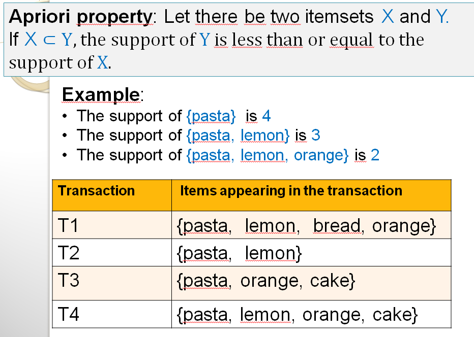
The Apriori algorithms is based on two important properties for reducing the search space. The first one is called the Apriori property (also called anti-monotonicity property). The idea is the following. Let there be two itemsets X and Y such that X is a subset of Y. The support of Y must be less than or equal to the support of X. In other words, if we have two sets of items X and Y such that X is included in Y, the number of transactions containing Y must be the same or less than the number of transactions containing X. Let me show you this with an example:
As you can see above, the itemset {pasta} is a subset of the itemset {pasta, lemon}. Thus, by the Apriori property the support of {pasta,lemon} cannot be more than the support of {pasta}. It must be equal or less than the support of {pasta}.
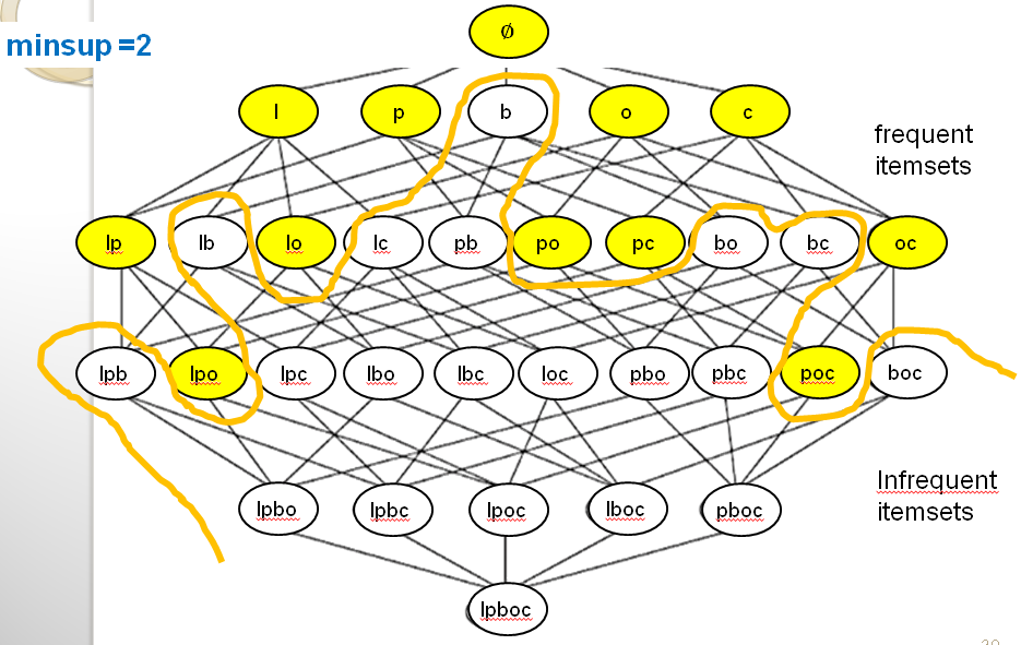
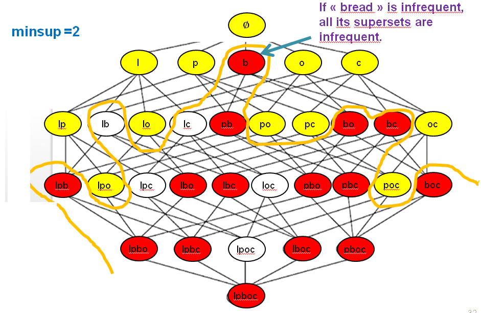
This property is very useful for reducing the search space, that is to avoid considering all possible itemsets when searching for the frequent itemsets. Let me show you this with some illustration. First, look at the following illustration of the search space:
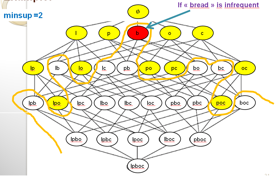
In the above picture, we can see that we can draw a line between the frequent itemsets (in yellow) and the infrequent itemsets (in white). This line is drawn based on the fact that all the supersets of an infrequent itemset must also be infrequent due to the Apriori property. Let me illustrate this more clearly. Consider the itemset {bread} which is infrequent in our example because its support is lower than the minsup threshold. That itemset is shown in red color below.
Then, based on the Apriori property, because bread is infrequent, all its supersets must be infrequent. Thus we know that any itemset containing bread cannot be a frequent itemset. Below, I have colored all these itemsets in red to make this more clear.
Thus, the Apriori property is very powerful. When an algorithm explores the search space, if it finds that some itemset (e.g. bread) is infrequent, we can avoid considering all itemsets that are supersets of that itemset (e.g. all itemsets containing bread).
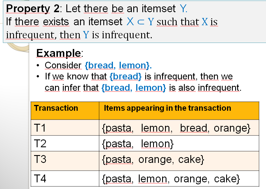
A second important property used in the Apriorialgorithm is the following. If an itemset contain a subset that is infrequent, it cannot be a frequent itemset. Let me show an example:
The property say that if we have an itemset such as {bread, lemon} that contain a subset that is infrequent such as {bread}, then the itemset cannot be frequent. In our example, since {bread} is infrequent, it means that {bread, lemon} is also infrequent. You may think that this property is very similar to the first property! Actually, this is true. It is just a different way of writing the same property. But it will be useful for explaining how the Apriorialgorithm works.
The Apriori algorithm
I will now explain how the Apriorialgorithm works with an example, as I want to explain it in an intuitive way. But first, let’s remember what is the input and output of the Apriori algorithm. The input is (1) a transaction database and (2) a minsup threshold set by the user. The output is the set of frequent itemsets. For our example, we will consider that minsup = 2 transactions.
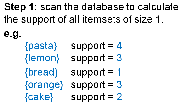
The Apriori algorithm is applied as follows. The first step is to scan the database to calculate the support of all items (itemsets containing a single items). The results is shown below
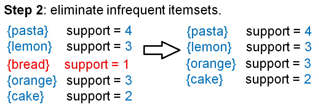
After obtaining the support of single items, the second step is to eliminate the infrequent itemsets. Recall that the minsup parameter is set to 2 in this example. Thus we should eliminate all itemsets having a support that is less than 2. This is illustrated below:
We thus now have four itemsets left, which are frequent itemsets. These itemsets are thus output to the user. All these itemsets each contain a single item.
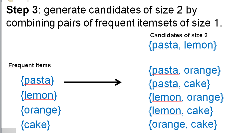
Next the Apriorialgorithm will find the frequent itemsets containing 2 items. To do that, the Apriorialgorithm combines each frequent itemsets of size 1 (each single item) to obtain a set of candidate itemsets of size 2 (containing 2 items). This is illustrated below:
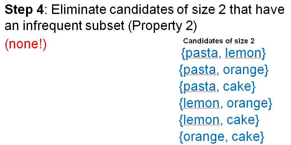
Thereafter, Apriori will determine if these candidates are frequent itemsets. This is done by first checking the second property, which says that the subsets of a frequent itemset must also be frequent. For the candidates of size 2, this would be done by checking if the subsets containing 1 items are also frequent. For the candidate itemsets of size 2, it is always true, so the Apriori algorithm does nothing.
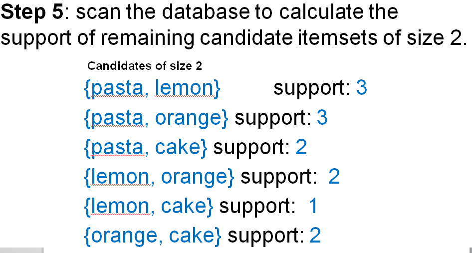
Then, the next step is to scan the database to calculate the exact support of the candidate itemsets of size 2, to check if they are reallyfrequent. The result is as follows.
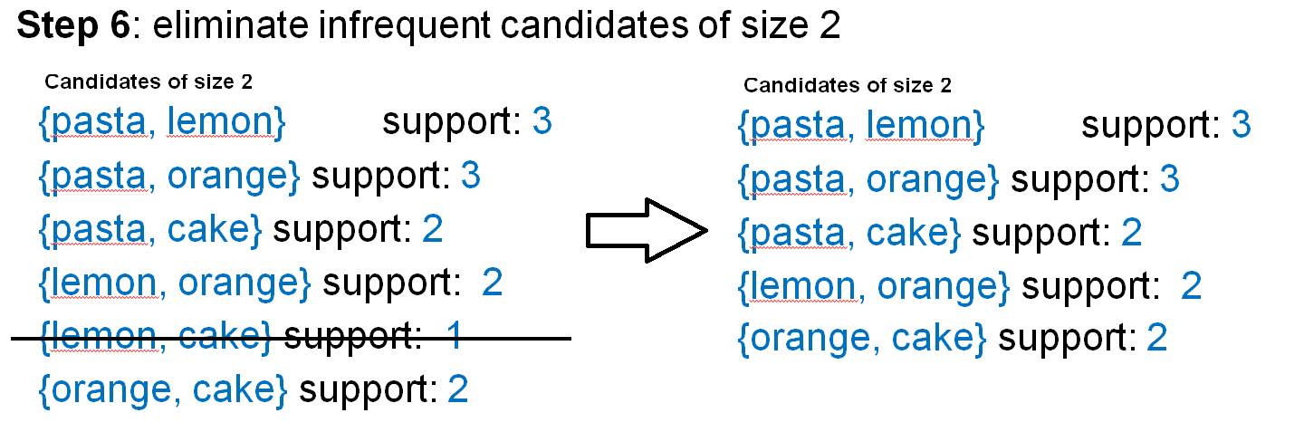
Based on these support values, the Apriorialgorithm next eliminates the infrequent candidate itemsets of size 2. The result is shown below:
As a result, there are only five frequent itemsets left. The Apriorialgorithm will output these itemsets to the user.
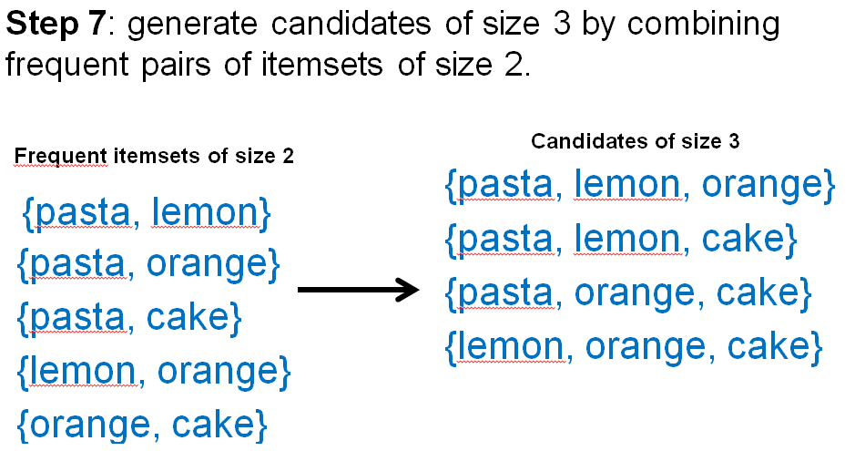
Next, the Apriorialgorithm will try to generate candidate itemsets of size 3. This is done by combining pairs of frequent itemsets of size 2. This is done as follows:
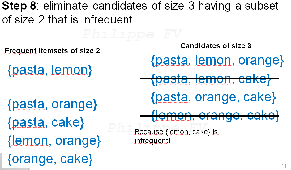
Thereafter, Apriori will determine if these candidates are frequent itemsets. This is done by first checking the second property, which says that the subsets of a frequent itemset must also be frequent. Based on this property, we can eliminate some candidates. The Apriorialgorithm checks if there exists a subset of size 2 that is not frequent for each candidate itemset. Two candidates are eliminated as shown below.
For example, in the above illustration, the itemset {lemon, orange, cake} has been eliminated because one of its subset of size 2 is infrequent (the itemset {lemon cake}). Thus, after performing this step, only two candidate itemsets of size 3 are left.
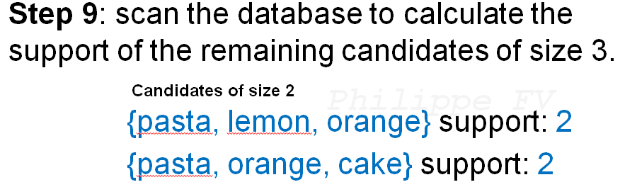
Then, the next step is to scan the database to calculate the exact support of the candidate itemsets of size 3, to check if they are really frequent. The result is as follows.
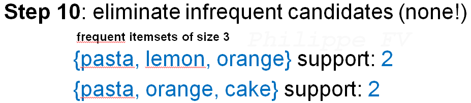
Based on these support values, the Apriorialgorithm next eliminates the infrequent candidate itemsets of size 3 o obtain the frequent itemset of size 3. The result is shown below:
There was no infrequent itemsets among the candidate itemsets of size 3, so no itemset was eliminated. The two candidate itemsets of size 3 are thus frequent and are output to the user.
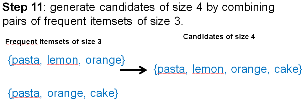
Next, the Apriorialgorithm will try to generate candidate itemsets of size 4. This is done by combining pairs of frequent itemsets of size 3. This is done as follows:
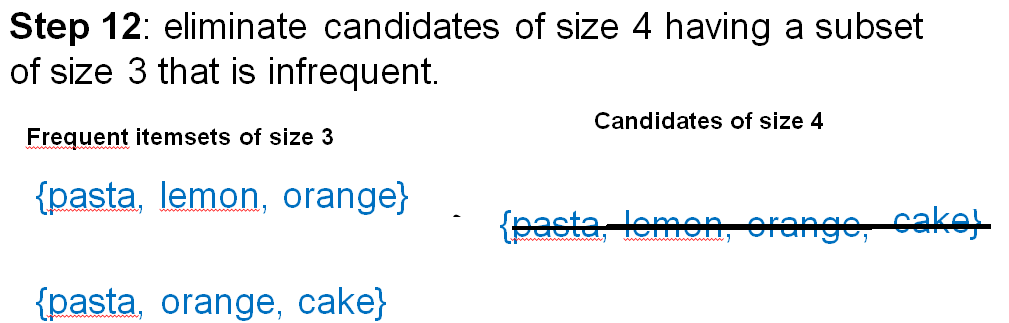
Only one candidate itemset was generated. hereafter, Apriori will determine if this candidate is frequent. This is done by first checking the second property, which says that the subsets of a frequent itemset must also be frequent. The Apriorialgorithm checks if there exist a subset of size 3 that is not frequent for the candidate itemset.
During the above step, the candidate itemset {pasta, lemon, orange, cake} is eliminated because it contains at least one subset of size 3 that is infrequent. For example, {pasta, lemon cake} is infrequent.
Now, since there is no more candidate left. The Apriori algorithm has to stop and do not need to consider larger itemsets (for example, itemsets containing five items).
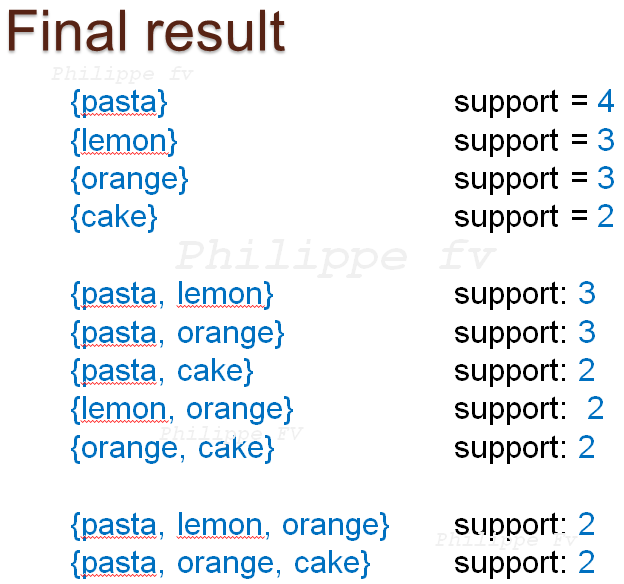
The final result found by the algorithm is this set of frequent itemsets.
Thus, the Apriorialgorithm has found 11 frequent itemsets. The Apriorialgorithm is said to be a recursive algorithm as it recursively explores larger itemsets starting from itemsets of size 1.
Now let’s analyze the performance of the Apriorialgorithm for the above example. By using the two pruning properties of the Apriorialgorithm, only 18 candidate itemsets have been generated. However, there was 31 posible itemsets that could be formed with the five items of this example (by excluding the empty set). Thus, thanks to its pruning properties the Apriorialgorithm avoided considering 13 infrequent itemsets. This may not seems a lot, but for real databases, these pruning properties can make Apriori quite efficient.
It can be proven that the Apriorialgorithm is complete (that it will find all frequent itemsets in a given database) and that it is correct (that it will not find any infrequent itemsets). However, I will not show the proof here, as I want to keep this blog post simple.
Technical details
Now, a good question is how to implement the Apriorialgorithm. If you want to implement the Apriorialgorithm, there are more details that need to be considered. The most important one is how to combine itemsets of a given size k to generate candidate of a size k+1.
Consider an example. Let’s say that we combine frequent itemsets containing 2 items to generate candidate itemsets containing 3 items. Consider that we have three itemsets of size 2 : {A,B}, {A,E} and {B,E}.
A problem is that if we combine {A,B} with {A,E}, we obtain {A,B,E}. But if we combine {A,E} with {B,E}, we also obtain {A,B,E}. Thus, as shown in this example, if we combine all itemsets of size 2 with all other itemsets of size 2, we may generate the same itemset several times and this will be very inefficient.
There is a simple trick to avoid this problem. It is to sort the items in each itemset according to some order such as the alphabetical order. Then, two itemsets should only be combined if they have all the same items except the last one.
Thus, {A,B} and {A,E} can be combined since only the last item is different. But {B,E} and {A,E} cannot be combined since some items are different that are not the last item of these itemsets. By doing this simple strategy, we can ensure that Apriori will never generate the same itemset more than once.
I will not show the proof to keep this blog post simple. But it is very important to use this strategy when implementing the Apriorialgorithm.
How is the performance of the Apriori algorithm?
In general the Apriorialgorithm is much faster than a naive approach where we would count the support of all possible itemsets, as Apriori will avoid considering many infrequent itemsets.
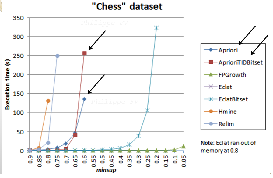
The performance of Apriori can be evaluated in real-life in terms of various criteria such as the execution time, the memory consumption, and also its scalability (how the execution time and memory usage vary when increasing the amount of data). Typically, researchers in the field of data mining will perform numerous experiments to evaluate the performance of an algorithm in comparison to other algorithms. For example, here is a simple experiment that I have done to compare the performance of Apriori with other frequent itemset mining algorithms on a dataset called “Chess“.
In that experiment, I have varied the minimum support threshold to see the influence on the execution time of the algorithms. As the threshold is set lower, more patterns need to be considered and the algorithms become slower. It can be seen that Apriori performs quite well but is still much slower than other algorithms such as Eclat and FPGrowth. This is normal since the Apriorialgorithm actually has some limitations that have been addressed in newer algorithms. For example, Apriori is an algorithm that can generate candidate itemsets that do not exist in the database (have a support of 0). More recent algorithms such as FPGrowth are designed to avoid this problem. Besides, note that here, I just show results on a single dataset. To perform a complete performance comparison, we should consider more than a single dataset. But I just show this as an example in this blog post. The experiment shown here was run with the SPMF data mining software which offers open-source implementations of Apriori and many other pattern mining algorithms in Java.
Source code and more information about Apriori
In this blog post, I have aimed at giving a brief introduction to the Apriori algorithm. I did not discuss optimizations, but there are many optimizations that have been proposed to efficiently implement the Apriori algorithm.
If you want to know more about Apriori, you could read the original paper by Agrawal published in 1993:
Rakesh Agrawal and Ramakrishnan Srikant Fast algorithms for mining association rules. Proceedings of the 20th International Conference on Very Large Data Bases, VLDB, pages 487-499, Santiago, Chile, September 1994.
To try Apriori, you can obtain a fast implementation of Apriori as part of the SPMF data mining software, which is implemented in Java under the GPL3 open-source license. The source code of Apriori in SPMF is easy to understand, fast, and lightweight (no dependencies to other libraries).
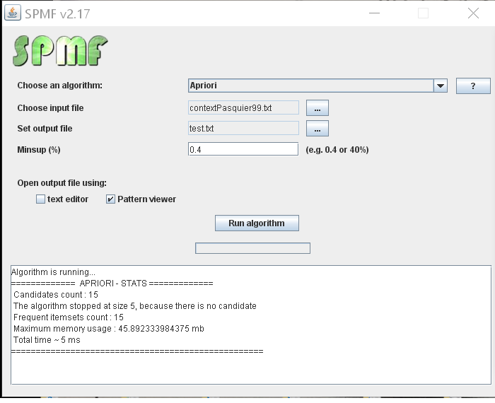
On the website of SPMF, examples and datasets are provided for running the Apriorialgorithm, as well as more than 100 other algorithms for pattern mining. The source code of algorithms in SPMF has no dependencies to other libraries and can be easily integrated in other software. The SPMF software also provides a simple user-interface for running algorithms:
Besides, if you want to know more about frequent itemset mining, I recommend to read my recent survey paper about itemset mining . It is easy to read and goes beyond what I have discussed in this blog post. The survey paper is more formal, gives pseudocode of Apriori and other algorithms, and also discusses extensions of the problem of frequent itemset mining and research opportunities.
Hope you have enjoyed this blog post! 😉
—
Philippe Fournier-Viger is a professor of computer science and founder of the SPMF data mining library.
On July 20 2017, I received an e-mail from a company called Clarivate Analytics Trademark Enforcement ( legal@ip-clarivateanalytics.com ) about copyright infringement for the Journal Citation Reports, a product by Thomson Reuters.
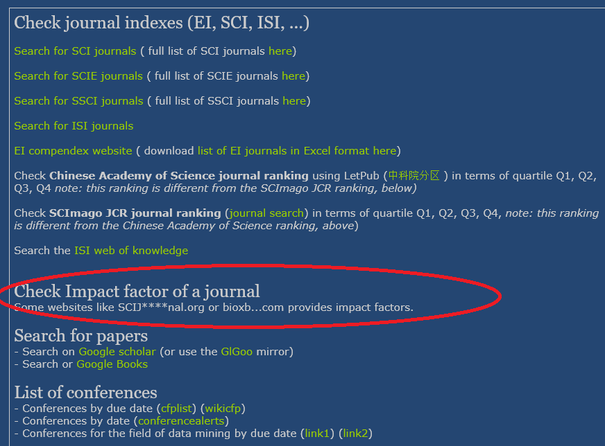
They contact with me because a few years ago I have created a webpagethat provides a list of useful links for researchers such as how to check if a journal is indexed by SCI, SCIE, IS, etc. It is a very simple webpage that donot host any copyright data, and is very useful for researchers. You can see a screenshot below:
Copryight claim
So what is the problem with this webpage? Well, the company did not like that I linked to two websites called SCIJ***nal.org and bioxb…com that provide the impactfactors of journals, which is a very useful information for researchers. They asked me to remove these two links as these websites apparently contain copyrighted data (the impact factors).
It should be clear that I donot host this data on my website, and I donot own these two websites either. Thus I am not responsible for their content. However, I have still decided to censor the links as you can see above, although I probably donot have to since linking to a website is generally not considered copyright infridgment.
A problem for academia
So what does this tells us about Thomson Reuters? I think that they would expect every researcher to pay to access the impact factors. But not all universities have the funding to pay to access this data, which is very inconvenient for young researchers or people working in small universities or less developed countries. To avoid such problems, I think that as researchers, we should try to move away from impact factors provided by a company. An impact factor is basically just calculated using some simple math formula using data provided by journals. There should be a way to have alternatives to these impactfactors that are not calculated or owned by a company.
The Streisand effect
Besides, can they really expect to censor links to these two websites all over the Internet? In the past, many people have failed to do this, and this has backfired. For example, there is the well known Streisand effect where the fact of trying to hide something makes it even more popular.
This is all I wanted to write for today. Just wanted to share this story.
—
By the way, all the names mentioned in this blog posts belong to the respective companies.
Many researchers wish to produce high quality papers and have a great research impact. But how? In a previous blog post, I have discussed how the “blue ocean strategy” can be applied to publish in top conference/journal. In this blog post, I will discuss another important concept for producing high impact research, which is to consider the opportunity cost of research.
Opportunity cost
The concept of opportunity cost is widely used in the field of economy. I will explain this concept and then explain how it can be applied to research. Consider a situation where you must choose between several mutually exclusive choices C1, C2, … Cn. If you choose a choice Cx, then you cannot choose the other choices because they are mutually exclusive with Cx. Thus, by making a choice Cx, you may be getting some benefits, but you may miss other benefits that could be obtained when making other choices. In other words, when we make a choice in a given situation, we not only get the rewards or benefits that goes with that choice but we also lose other benefits that we could have obtained if we had made other choices. The opportunity cost for making a choice Cx is thus the lost of benefits caused by not making other alternative choices.
Applying the concept of opportunity cost in research
The concept of opportunity cost is simple but very useful in many domains, and considering it allows to take better decisions. When making a choice between multiple alternatives, we should not only think about the direct benefits of that choice but also at the missed opportunities from other alternative choices (the opportunitycost).
How does that applies to research? Well, in research, a researcher has multiple resources (times, money, students). In terms of time, when a researcher decides to spend time on a given project, he may as a result not have time to work on alternative research projects. Thus, given the limited amount of time that a researcher has, he must carefully choose between multiple research opportunities to maximize his benefits.
For example, it is tempting for several young researchers to write several papers with simple an unoriginal ideas, just to publish papers as quickly as possible. This may seems like a good idea in the short term. However, the hidden opportunitycost of doing so is that the time spent on writing these simple papers cannot be spent to work on better research ideas that take more time to develop but may result in a higher impact on the long term.
Thus, from the perspective of opportunity cost, a researcher should try to choose carefully the research projects that are promising and spend more time to develop these projects and make good papers out of it, rather than to try to write as many papers as possible.
From my experience, even the most simple conference papers requires at least 1 or 2 weeks of work that could be spend on better research projects. The fastest paper that I have written for a conference was done in about 1 week, several years ago. But still, even if it only takes a week, one should not forget that additional time needs to be spent to travel, prepare a PowerPoint, and present the paper at a conference. Thus, totally, the cost in terms of time for a quick conference paper may still add up to two weeks or more. And then, as explained, the opportunitycost of writing a simple paper is that one may not have enough time to work on better or more promising research ideas. Thus, in recent years, I have shifted my focus to target better conferences and journals and focus less on smaller conferences. I write less papers but these papers are of higher quality and can have a greater impact.
Of course, many other factors must be considered to publish high quality papers such as the choice of a good research topic. But in this blog post, I wanted to highlight the concept of opportunitycost.
Conclusion
In this blog post, I have highlighted how opportunitycost is applicable to research in academia. I personally think that it is an important concept, as many researchers are tempted to publish as many papers as possible without focusing much on quality, and often without realizing that that time could be spent on better research ideas. But producing high impact research requires to spend a considerable amount of time. Thus, one should carefully chose to spend more time on promising projects, rather than focusing too much on quantity. Besides time, the concept of opportunitycost is also applicable to other kinds of resources such as funding and students.
If you like this blog, you can subscribe to the RSS Feed or my Twitter account (https://twitter.com/philfv) to get notified about future blog posts
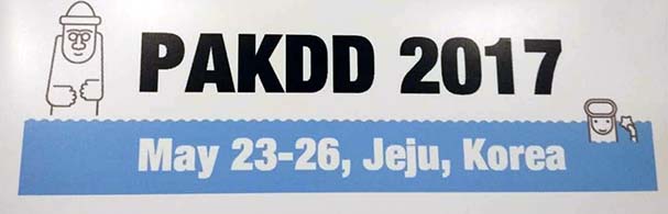
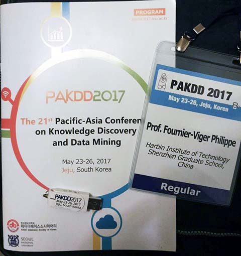
This week, I have attended the PAKDD 2017 conference in Jeju Island, South Korea, this week, from the 23 to 26th May. PAKDDis the top data mining conference for the asia-pacific region. It is held every year in a different pacific-asian country. In this blog post, I will write a briefreport about the conference.
Conference location
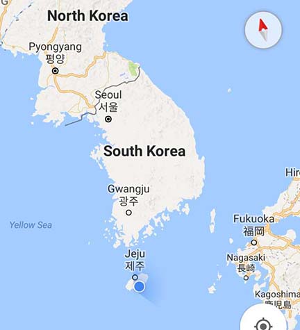
The PAKDD conference was held in the city of Seogwipo on Jeju island, a beautiful island in South Korea, which is famous for tourism, especially in Asia. Here is a map of the location.
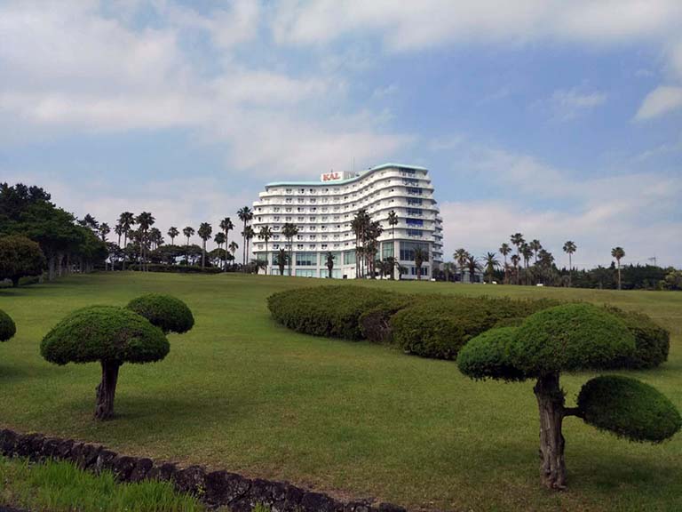
In particular, the PAKDDconference was held at the Seogwipo KAL hotel.
The hotel was well-chosen. It is about 1 km from the city, beside the sea.
Conference proceedings
The proceedings of the PAKDD 2017 conference are published by Springer in the Lecture Notes in Artificial Intelligence series. This ensures a good visibility to the papers published in the proceedings, which are indexed in the main computer science indexes such as DBLP.
The proceedings were given on a USB drive (4 Gb) rather than as a book, as many other conferences have been doing in recent years. Personally, I like to have proceedings as books, but USB drives are probably more friendly for the environment.
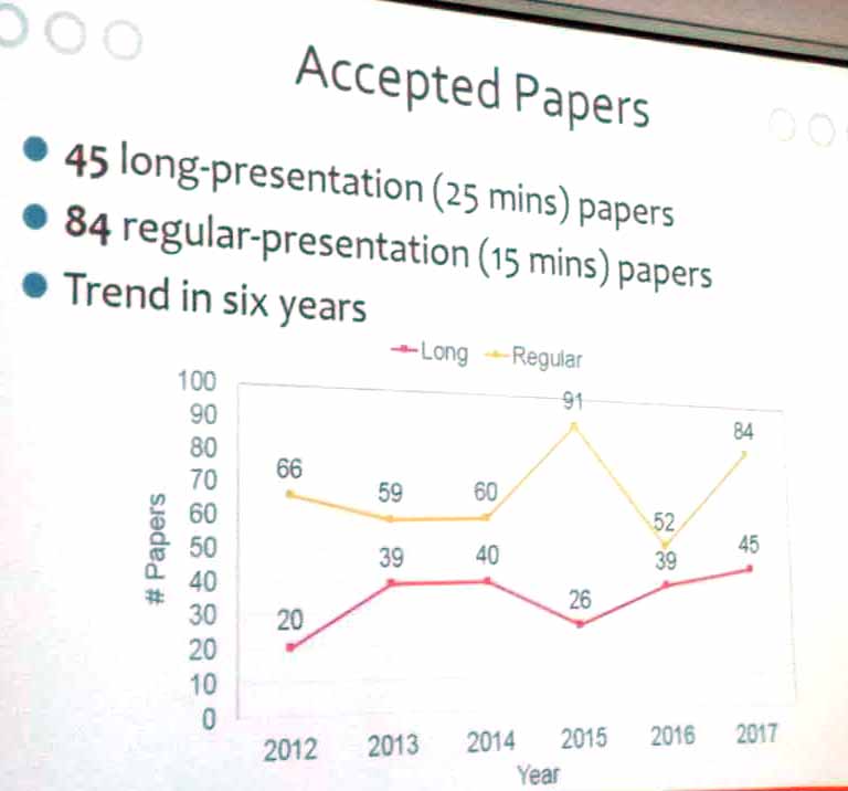
In general the quality of the papers at PAKDD conferences is good. This year, 458 papers were submitted. Among those, 45 papers were accepted as long papers and 84 as short papers. Thus, the global acceptance rate was about 28%.
Below, I present various slides from the opening ceremony presentation, which provides information about the PAKDDconference this year.
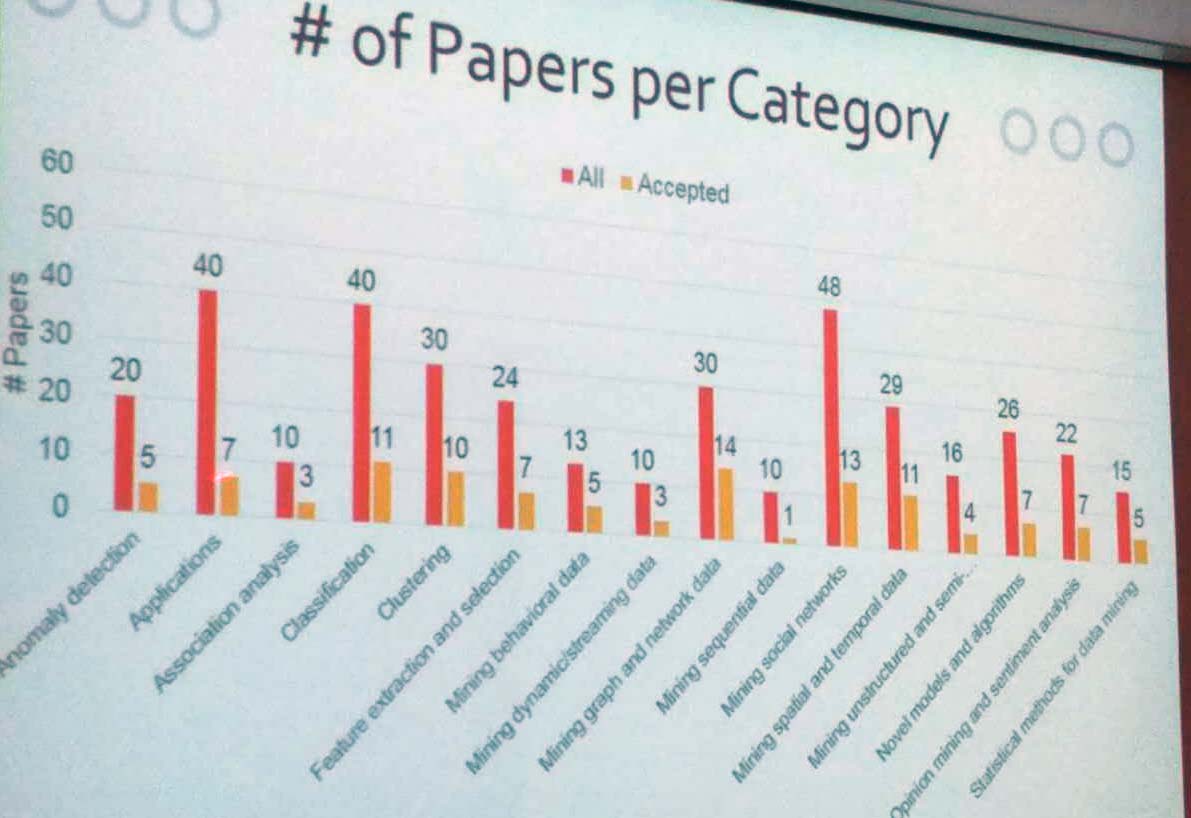
The number of papers per category (submitted / accepted) is shown below. It is interesting to see that a large amount of applications and social network papers have been rejected. And for the topic of sequential data, only 1 paper out of 10 was accepted.
2) The number of accepted long and short papers at PAKDD forthe last six years is presented below.
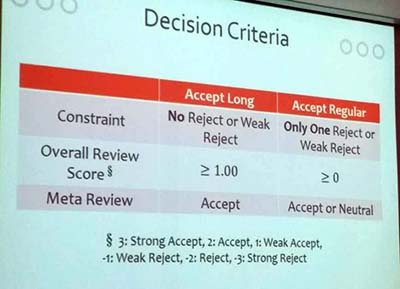
3) The decision criteria for accepting a paper at PAKDD are shown below.
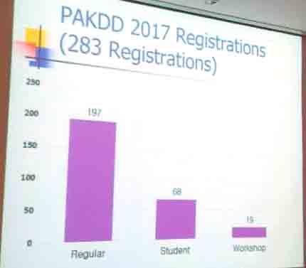
4) There was 283 persons who have registered for PAKDD this year.
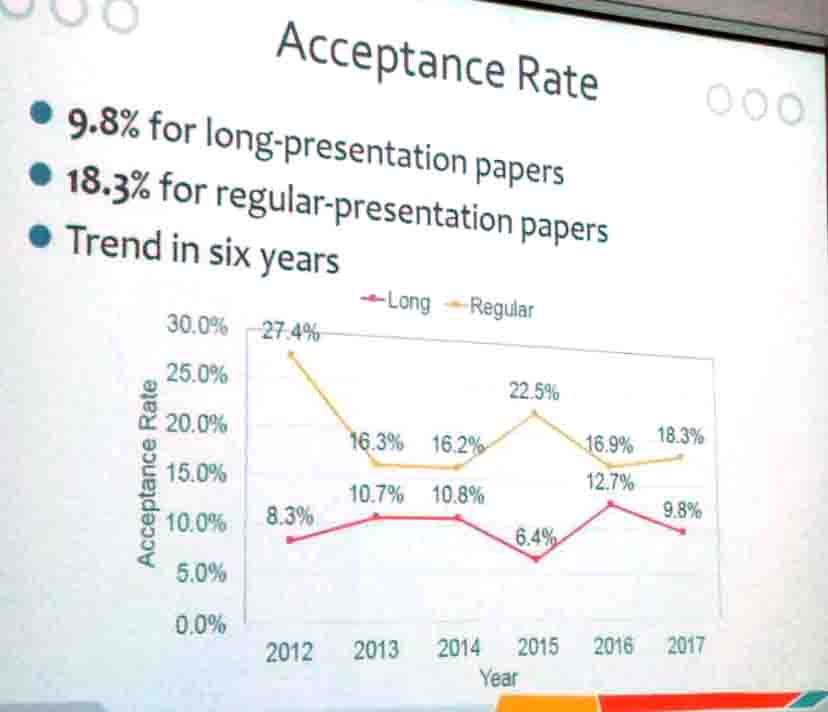
5) The acceptance rate of long and short papers at PAKDD during the last six years
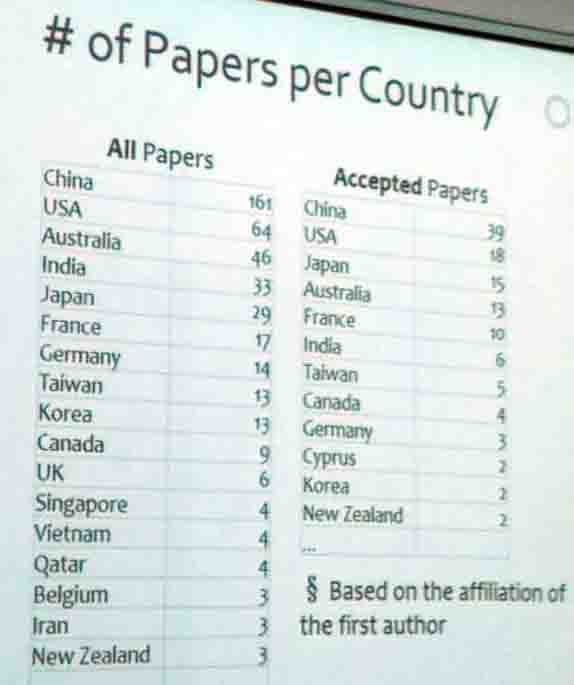
6) The number of submitted vs accepted papers by country this year. We can observe that China has the largest number of papers accepted and submitted.
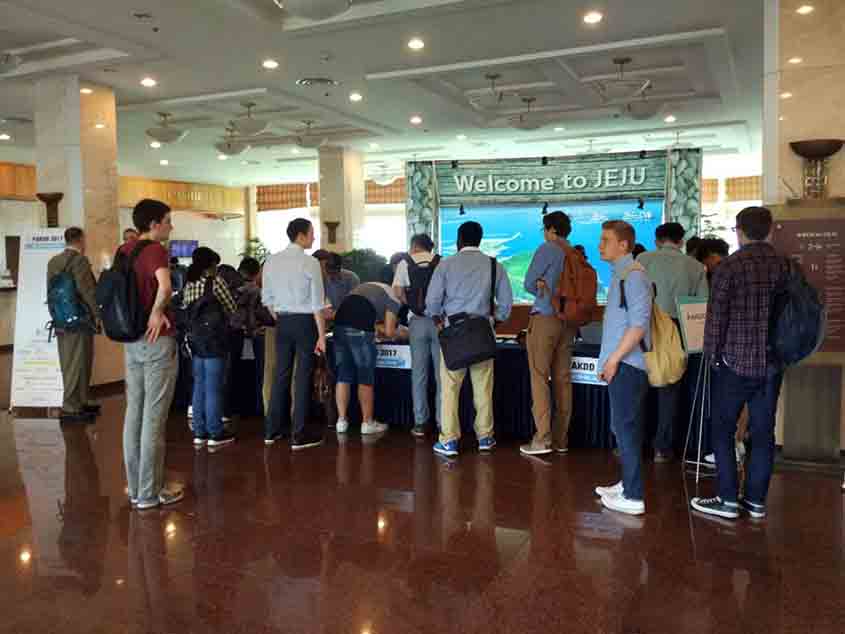
Day 1 – workshops and tutorials, reception
On the first day, the registration started at 8:00 AM.
It was then followed by various workshops and tutorials. I have attended a workshop about Biologically Inspired Data Mining, a popular topic, which covers the applications of algorithms such as neural networks, bee swarm optimization, genetic algorithms, and ant colony optimization, to solve data mining problems. Evolutionary algorithms are quite interesting as they can find approximate solutions to data mining problems that are quite good solutions, while running much faster than traditional algorithms that find an optimal solution. There was also some tutorials that I did not attend on information retrieval, recommender systems and tensor analysis. Besides, there was workshops on security, business process management, and sensor data analytics.
In the evening, there was a reception, which was a good opportunity for discussing with other researchers.
Day 2 – main conference, opening ceremony
There was an opening ceremony, followed by a keynote by Sang Kyun Cha from the Seoul National University of Korea. The keynote was about a potential fourth industrial revolution that would occurs due to the growth of AI-based services and big data technologies. This would lead to a need for more skilled workers such as engineers or “data scientists”. The talk was interesting but personally I prefer talks that are a little bit more technical. After that, there was multiple sessions of paper presentations.
Besides technical sessions, I also discussed with some representatives from Nvidia who were promoting a new supercomputer specially designed for training deep learning neural networks. It is called NVIDIA DGX-1 and costs around 200,000 $ USD. According to the promotional material, this computer has a eight Tesla P100 GPUs, each with 16 GB of memory, a total of 28672 NVIDIAN CUDA cores, and two dual 20-core Intel Xeon E5-2698 v4 2.2 Ghz processors. But what is the most interesting is that this GPU based system is claimed to be 250 times faster than a conventional CPU-only server for deep learning. I saw that there is also a similar product by IBM called the IBM Minsky, also equipped with NVidia GPUs. This is especially interesting for those working on deep learning related topics.
NVidia DGX1
Day 3 – main conference, excursion, banquet
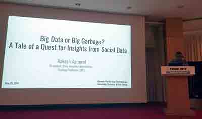
On the third day of the conference, there was a keynote speech by Rakesh Agrawal, a senior researcher, who is one of the founder of data mining. The talk was about the usage of social data.. The main question addressed in this talk was whether social data from websites such as Twitter is garbage or it can be useful for businesses. R. Agrawal presented a project that he carried a few years ago at Microsoft where he analyzed Twitter data to study the opinion of people about Microsoft products. He also described a work where he compared the results of the Bing and Google search engines, and the result obtained when searching using social data rather than traditional search engines. The conclusion was that social data is certainly useful. R. Agrawal also gave some advices that young researchers should try to choose good research topics that are useful and can have an impact rather than just focusing on publishing a paper as quickly as possible.
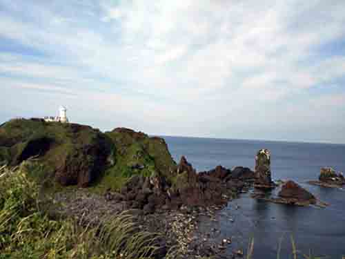
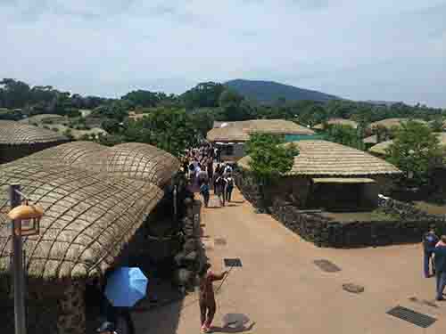
On the afternoon, there was an excursion to Seopjikoji beach, Seongsan Sunrise Peak and Seongeup Folk Village.
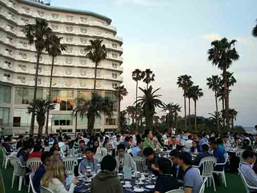
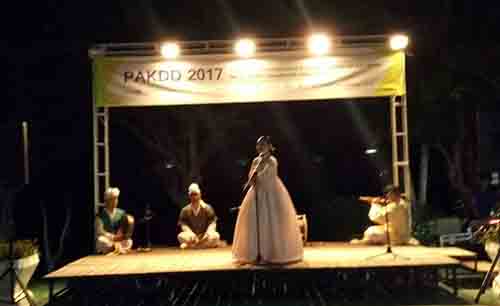
In the evening, there was a banquet at the Seogwipo KAL hotel, with a musical performance.
Day 4 – main conference, closing ceremony
On the fourth day, there was a keynote by Dacheng Tao, from the University of Sydney Australia about current challenges in artificial intelligence. It was followed by several technical sessions, a lunch and a closing ceremony.
Conclusion
The conference was quite interesting. I had the occasion to meet many interesting people from academia and also from industry (e.g. Microsoft, Yahoo, Adobe, Nvidia). PAKDD is not the largest conference in data mining but it is a quite good conference, especially for the asia-pacific region, and the quality of the papers is quite high. It was announced that next year, thePAKDD 2018 conference will be held in Melbourne, Australia. I will certainly try to attend it.
— Philippe Fournier-Viger is a professor of Computer Science and also the founder of the open-source data mining software SPMF, offering more than 120 data mining algorithms.