In this blog post, I will continue the discussion of how to write research papers. I will discuss the importance of writing a good abstract for research papers, common errors, and give some tips.

Why the abstract is important?
The abstract is often overlooked but it is one of the most important part of a paper. The purpose of the abstract is to provide a short summary of a paper. A potential reader will often only look at the abstract and title to decide to read a paper or not. A good abstract will increase the probability that a paper is read or cited, while a bad abstract will have the opposite effect.
The abstract is also very important because many papers are behind a paywall (a publisher will only provide the abstract and ask readers to pay to read the full paper).
What is the typical structure of an abstract?
The structure of an abstract is always more or less the same. Typically, it is a single paragraph, containing five parts:
- PART 1 (context): The first sentences talk about the context (background) of the paper from a very general perspective.
- PART 2 (problem): Then, a problem is mentioned and why it must be solved.
- PART 3 (limitations): Then, the abstract briefly mentions that solutions proposed in previous studies are insufficient to solve the problem due to some limitations. Thus, we need a new solution.
- PART 4 (contributions): Then, the abstract mentions the contributions of the paper, which is to propose a new solution, and what are the key features of that solution.
- PART 5 (results and conclusion): Then, one or two sentences are used to briefly mention the experiment results, and conclusion or implications that can be drawn from these results.
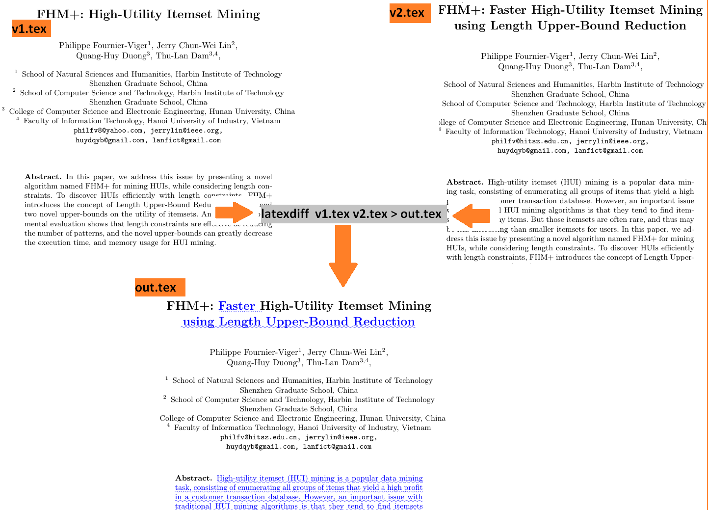
This type of structure gives a concise overview of the content of the paper. The next paragraph gives an example of an abstract, which adopts this structure, from the paper describing the EFIM algorithm:
PART 1: In recent years, high-utility itemset mining has emerged as an important data mining task. PART 2 and 3: However, it remains computationally expensive both in terms of runtime, and memory consumption. It is thus an important challenge to design more efficient algorithms for this task. PART 4: In this paper, we address this issue by proposing a novel algorithm named EFIM (EFficient high-utility Itemset Mining), which introduces several new ideas to more efficiently discover high-utility itemsets. EFIM relies on two new upper-bounds named revised sub-tree utility and local utility to more effectively prune the search space. It also introduces a novel array-based utility counting technique named Fast Utility Counting to calculate these upper-bounds in linear time and space. (… ) PART 5: An extensive experimental study on various datasets has shown that EFIM is in general two to three orders of magnitude faster than the state-of-art algorithms d2HUP, HUI-Miner, HUP-Miner, FHM and UP-Growth+ on dense datasets and performs quite well on sparse datasets. Moreover, a key advantage of EFIM is its low memory consumption.
There is typically a maximum length restriction for an abstract. For example, some journals may require no more than 200 words. For a very short abstract, the PARTS 1,2,3 can be made very short or ommitted to focus on PART 4 and 5. For example:
PART 1,2,3: High utility itemset mining has many applications but performance remains an important issue. PART 4: To address this problem, a novel algorithm named EFIM (EFficient high-utility Itemset Mining) is presented, which relies on two new upper-bounds to prune the search space, and a novel array-based utility counting technique. PART 5: Experiments have shown that EFIM has low memory consumption and is up to 50 times faster than state-of-art algorithms on dense datasets and performs quite well on sparse datasets.
For some other types of paper such as survey papers the structure is similar but some parts are omitted. Here is an example from a survey paper about frequent itemset mining:
PART 1: Itemset mining is an important subfield of data mining, which consists of discovering interesting and useful patterns in transaction databases. The traditional task of frequent itemset mining is to discover groups of items (itemsets) that appear frequently together in transactions made by customers. Although itemset mining was designed for market basket analysis, it can be viewed more generally as the task of discovering groups of attribute values frequently co-occurring in databases. Due to its numerous applications in domains such as bioinformatics, text mining, product recommendation, e-learning, and web click stream analysis, itemset mining has become a popular research area. PART 4: This paper provides an up-to-date survey that can serve both as an introduction and as a guide to recent advances and opportunities in the field. The problem of frequent itemset mining and its applications are described. Moreover, main approaches and strategies to solve itemset mining problems are presented, as well as their characteristics. Limitations of traditional frequent itemset mining approaches are also highlighted, and extensions of the task of itemset mining are presented such as high-utility itemset mining, rare itemset mining, fuzzy itemset mining and uncertain itemset mining. The paper also discusses research opportunities and the relationship to other popular pattern mining problems such as sequential pattern mining, episode mining, subgraph mining and association rule mining. Main open-source libraries of itemset mining implementations are also briefly presented.
Which verb tense should be used?
A good question is: Which verb tenses should be used in an abstract? Some general suggestions are:
- To describe previous studies, the past tense is used,
- To present general facts, the present tense is used
- To discuss the contributions of the paper or what the paper will present, the present tense is recommended (e.g. “This paper proposes an algorithm named …”) .
- If the abstract discusses some experimental results, the past tense is recommended (e.g. “Experiments have shown that…”)
Some common errors
I will now discuss six common errors found in abstracts:
- An abstract containing English errors. The title is the first thing that someone reads, and then it is the abstract before reading the whole paper. If a title or an abstract contains English errors, it may give a bad impression to readers.
- An abstract that does not accurately describe the content of the paper. Sometimes, only the abstract is available to the reader. If the abstract does not give a good overview of the paper, one may not try to access the full paper.
- An abstract that does not follow the typical structure and is not logically organized. A good abstract will follow the standard structure described in this post, to ensure that ideas are presented in a logical way.
- An abstract that contains abbreviations and acronyms. Generally, it is recommended to avoid using acronyms and abbreviations in an abstract since the reader may not be familiar with them. Moreover since abstracts are short, it is typically unnecessary to define abbreviations in an abstract.
- An abstract that contains citations, or refer to tables and figures. An abstract should not contain citations, except in some exceptional cases. Moreover, an abstract should never refer to figures or tables.
- An abstract that contains irrelevant details. Given that an abstract is often restricted to a maximum length, it is important to avoid wasting this space by discussing details that are not important. Thus, the abstract should be concisely written and focus on the key points of the paper.
A few tips
Here are a few additional tips about writing an abstract:
- Before writing, check if there is a maximum length constraint for the abstract, specified by the publisher.
- Think about your target audience and use appropriate keywords and expressions in your abstract to ensure that other people in your field can find your paper.
- A good way to learn how to write abstracts is to look at the abstracts of other papers in your field.
- Take your time to write an abstract. If necessary, show it to a peer and ask his opinion.
- If necessary, ask someone to proofread your abstract to remove all English errors.
- Write sentences that are not too long, and are concise.
- Several researchers prefer to write an abstract after all the other parts of the paper have been written. This make sense since the abstract is a summary of the content of a paper. However, do not only copy and paste sentences from the paper to write the abstract. You may reuse some parts of sentences from the paper but you should adapt them.
Conclusion
That is all for this topic. I hope that you have enjoyed this blog post. I will continue discussing writing research papers in the next blog post. Looking forward to read your opinion and comments in the comment section below!
—-
Philippe Fournier-Viger is a professor of Computer Science and also the founder of the open-source data mining software SPMF, offering more than 145 data mining algorithms.