
Today, I will show how to draw a sequence in Latex using the TIKZ package. A sequence is an ordered list of symbols. I often draw sequences for my research paper about sequential pattern mining or episode mining. To draw a sequence, I first import the TIKZ package by adding this line in the section for packages:
\usepackage{tikz}
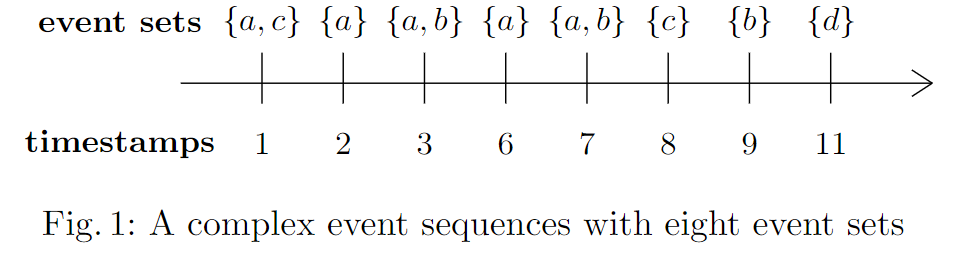
Example 1. To draw a sequence in a figure that looks like this:
I use this code:
\begin{figure}[ht]
\centering
\begin{tikzpicture}
%timeline
\draw (-0.4,0) -- (7,0);
% The labels
\node[] at (-1,0.6) {\textbf{event sets}};
\node[] at (-1,-0.6) {\textbf{timestamps}};
% first element
\draw (0.4,-0.2) -- (0.4,0.3); \node[] at (0.4,0.6) {${a,c}$}; \node[] at (0.4,-0.6) {$1$};
% second element
\draw (1.2,-0.2) -- (1.2,0.3); \node[] at (1.2,0.6) {${a}$}; \node[] at (1.2,-0.6) {$2$};
% third element
\draw (2,-0.2) -- (2,0.3); \node[] at (2,0.6) {${a,b}$}; \node[] at (2,-0.6) {$3$};
% next element
\draw (2.8,-0.2) -- (2.8,0.3); \node[] at (2.8,0.6) {${a}$}; \node[] at (2.8,-0.6) {$6$};
% next element
\draw (3.6,-0.2) -- (3.6,0.3); \node[] at (3.6,0.6) {${a,b}$}; \node[] at (3.6,-0.6) {$7$};
% next element
\draw (4.4,-0.2) -- (4.4,0.3); \node[] at (4.4,0.6) {${c}$}; \node[] at (4.4,-0.6) {$8$};
% next element
\draw (5.2,-0.2) -- (5.2,0.3); \node[] at (5.2,0.6) {${b}$}; \node[] at (5.2,-0.6) {$9$};
% next element
\draw (6,-0.2) -- (6,0.3); \node[] at (6,0.6) {${d}$}; \node[] at (6,-0.6) {$11$};
% The arrow
\draw (6.8,-0.13) -- (7,0);
\draw (6.8,0.13) -- (7,0);
\end{tikzpicture}
\caption{A complex event sequence with eight event sets}
\label{CES}
\end{figure}
You could improve upon this using other options in Tikz to add colors, etc.
Example 2: Another version of that example, with more timestamps:

The Latex code:
\begin{figure}[ht]
  %  \centering
%    \includegraphics[width=0.7\textwidth]{SEQ.pdf}
%\begin{figure}[ht]%
\centering
\begin{tikzpicture}
%timeline
\draw (-0.4,0) -- (10,0);
% The labels
\node[] at (-1,0.6) {\textbf{event sets}};
\node[] at (-1,-0.6) {\textbf{timestamps}};
% first element
\draw (0.4,-0.2) -- (0.4,0.3); \node[] at (0.4,0.6) {$\{c\}$}; \node[] at (0.4,-0.6) {$t_1$};
% second element
\draw (1.2,-0.2) -- (1.2,0.3); \node[] at (1.2,0.6) {$\{a,b\}$}; \node[] at (1.2,-0.6) {$t_2$};
% third element
\draw (2,-0.2) -- (2,0.3); \node[] at (2,0.6) {$\{d\}$};
\node[] at (2,-0.6) {$t_3$};
% next element
\draw (2.8,-0.2) -- (2.8,0.3); \node[] at (2.8,0.6) {}; \node[] at (2.8,-0.6) {$t_4$};
% next element
\draw (3.6,-0.2) -- (3.6,0.3); \node[] at (3.6,0.6) {$\{a\}$}; \node[] at (3.6,-0.6) {$t_5$};
% next element
\draw (4.4,-0.2) -- (4.4,0.3); \node[] at (4.4,0.6) {$\{c\}$}; \node[] at (4.4,-0.6) {$t_6$};
% next element
\draw (5.2,-0.2) -- (5.2,0.3); \node[] at (5.2,0.6) {$\{b\}$}; \node[] at (5.2,-0.6) {$t_7$};
% next element
\draw (6,-0.2) -- (6,0.3); \node[] at (6,0.6) {$\{d\}$}; \node[] at (6,-0.6) {$t_8$};
% next element  9
\draw (7,-0.2) -- (7,0.3); \node[] at (7,0.6) {}; \node[] at (7,-0.6) {$t_9$};
% next element 10
\draw (8,-0.2) -- (8,0.3); \node[] at (8,0.6) {$\{a,b,c\}$}; \node[] at (8,-0.6) {$t_{10}$};
% next element 11
\draw (9,-0.2) -- (9,0.3); \node[] at (9,0.6) {$\{a\}$}; \node[] at (9,-0.6) {$t_{11}$};
% The arrow
\draw (9.8,-0.13) -- (10,0);
\draw (9.8,0.13) -- (10,0);
\end{tikzpicture}
    \caption{A complex event sequence}
    \label{figseq}
\end{figure}
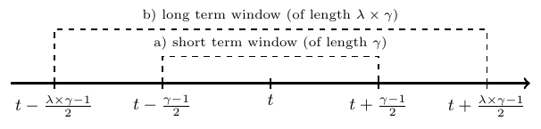
Example 3. Here is a more complicated example. To draw a sequence that looks like this:
I use this code:
\begin{figure}
\centering
%%%%%%%%%%%%%%%%%%%%%%%%%%%%
\begin{tikzpicture}[xscale=8]
\draw[-][draw=black, very thick] (-0.1,0) -- (.5,0);
\draw[->][draw=black, very thick] (.5,0) -- (1.1,0);
%\draw [thick] (0,-.1) node[below]{0} -- (0,0.1);
\draw [thick] (0.25,-.1) node[below]{$t-\frac{\gamma-1}{2}$} -- (0.25,0.1);
\draw [thick] (0,-.1) node[below]{$t-\frac{\lambda\times\gamma-1}{2}$} -- (0,0.1);
%%%%  WINDOW A
\draw [thick, dashed] (0.25,0) -- (0.25,.5) -- (.5,.5) node[above]{
\scriptsize a) short term window (of length $\gamma$)
} -- (0.75,.5) -- (0.75,0) ;
\draw [thick, dashed] (0,0) -- (0,1) -- (.5,1) node[above]{
\scriptsize b) long term window (of length $\lambda \times \gamma $)
} -- (1,1) -- (1,0) ;
\draw [thick] (0.5,-.1) node[below]{$t$} -- (0.5,0.1);
\draw [thick] (0.75,-.1) node[below]{$t+\frac{\gamma-1}{2}$} -- (0.75,0.1);
\draw [thick] (1,-.1) node[below]{$t+\frac{\lambda\times\gamma-1}{2}$} -- (1,0.1);
%\draw [thick] (1,-.1) node[below]{1} -- (1,0.1);
\end{tikzpicture}
%\caption{The windows for calculating the a) short term and b) long term moving average utility  for a timestamp $t$.}

\end{figure}
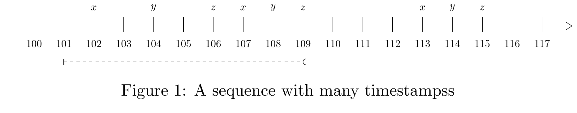
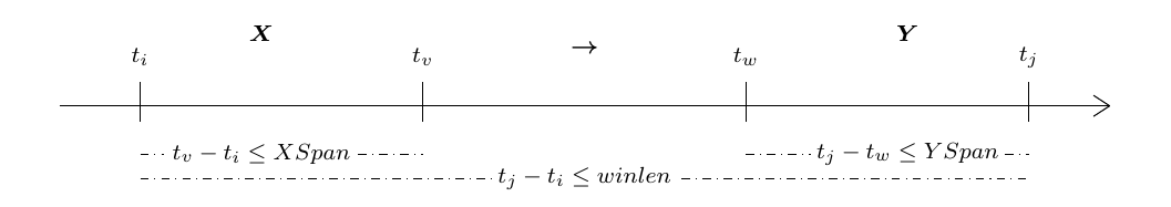
Example 4. And to draw a sequence like this that display some interval:
I use that code:
\begin{figure}[ht]
\centering
	\resizebox{\columnwidth}{!}{
\begin{tikzpicture}
%timeline
\draw (0,0) -- (19,0);
% first element
\draw (1,-0.2) -- (1,0.3);	 \node[] at (1,0.6) { }; 	\node[] at (1,-0.6) {100};
\draw (2,-0.2) -- (2,0.3);	 \node[] at (2,0.6) { }; 	\node[] at (2,-0.6) {101};
% Window 1
\draw[thick] (2,-1.1) -- (2,-1.3); \draw[dashed] (2,-1.2) -- (10,-1.2); \draw(10.1,-1.1) arc (90:270:0.1);
%%%%
\draw (3,-0.2) -- (3,0.3);	 \node[] at (3,0.6) {$x$}; 	\node[] at (3,-0.6) {102};
\draw (4,-0.2) -- (4,0.3);	 \node[] at (4,0.6) { }; 	\node[] at (4,-0.6) {103};
\draw (5,-0.2) -- (5,0.3);	 \node[] at (5,0.6) {$y$}; 	\node[] at (5,-0.6) {104};
\draw (6,-0.2) -- (6,0.3);	 \node[] at (6,0.6) { }; 	\node[] at (6,-0.6) {105};
\draw (7,-0.2) -- (7,0.3);	 \node[] at (7,0.6) {$z$}; 	\node[] at (7,-0.6) {106};
\draw (8,-0.2) -- (8,0.3);	 \node[] at (8,0.6) {$x$}; 	\node[] at (8,-0.6) {107};
\draw (9,-0.2) -- (9,0.3);	 \node[] at (9,0.6) {$y$}; 	\node[] at (9,-0.6) {108};
\draw (10,-0.2) -- (10,0.3);	 \node[] at (10,0.6) {$z$}; 	\node[] at (10,-0.6) {109};
\draw (11,-0.2) -- (11,0.3);	 \node[] at (11,0.6) { }; 	\node[] at (11,-0.6) {110};
\draw (12,-0.2) -- (12,0.3);	 \node[] at (12,0.6) { }; 	\node[] at (12,-0.6) {111};
\draw (13,-0.2) -- (13,0.3);	 \node[] at (13,0.6) { }; 	\node[] at (13,-0.6) {112};
\draw (14,-0.2) -- (14,0.3);	 \node[] at (14,0.6) {$x$}; 	\node[] at (14,-0.6) {113};
\draw (15,-0.2) -- (15,0.3);	 \node[] at (15,0.6) {$y$}; 	\node[] at (15,-0.6) {114};
\draw (16,-0.2) -- (16,0.3);	 \node[] at (16,0.6) {$z$}; 	\node[] at (16,-0.6) {115};
\draw (17,-0.2) -- (17,0.3);	 \node[] at (17,0.6) {}; 	\node[] at (17,-0.6) {116};
\draw (18,-0.2) -- (18,0.3);	 \node[] at (18,0.6) { }; 	\node[] at (18,-0.6) {117};

% The arrow
\draw (18.8,-0.13) -- (19,0);
\draw (18.8,0.13) -- (19,0);
\end{tikzpicture}
}
\caption{A sequence with many timestamps}
\label{CES}
\end{figure}
Example 5
And here is another example:
And here is the Latex code:
\begin{tikzpicture}
%timeline
\draw (-2,0) -- (11,0);
% first interval
\draw (-1,-0.2) -- (-1,0.3);
\draw (2.5,-0.2) -- (2.5,0.3);
\node[] at (-1,0.6) {$t_i$};
\node[] at (0.5,0.9) {$ \boldsymbol X$};
\node[] at (0.5,-0.6) {$t_v - t_i \leq XSpan$};
\draw [thin,dash dot] (-1,-0.6) -- (-0.7,-0.6);
\draw [thin,dash dot] (1.7,-0.6) -- (2.5,-0.6);
% second interval
% \draw (3,0) -- (6.5, 0);
\draw (6.5,-0.2) -- (6.5,0.3);
\node[] at (2.5,0.6) {$t_v$};
\node[] at (6.5,0.6) {$t_w$};
\node[] at (4.5,0.7) {$ \boldsymbol \rightarrow$};
\node[] at (4.5,-0.9) {$t_j - t_i \leq winlen$};
\draw [thin,dash dot] (-1,-0.9) -- (3.4,-0.9);
\draw [thin,dash dot] (5.7,-0.9) -- (10,-0.9);
%third interval
% \draw (6.5,0) -- (10,0);
\draw (6.5,-0.2) -- (6.5,0.3);
\draw (10,-0.2) -- (10,0.3);
\node[] at (10,0.6) {$t_j$};
\node[] at (8.5,0.9) {$ \boldsymbol Y$};
\node[] at (8.5,-0.6) {$t_j - t_w \leq YSpan$};
\draw [thin,dash dot] (6.5,-0.6) -- (7.3,-0.6);
\draw [thin,dash dot] (9.7,-0.6) -- (10,-0.6);
%arrow
\draw (10.8,-0.13) -- (11,0);
\draw (10.8,0.13) -- (11,0);
\end{tikzpicture}
Bonus
Besides, as a bonus, if I want to write a sequence using Latex math notation in a paragraph, I write like this:
$S=\langle ({a,c}, $ $ 1),$ $
({a},2),$ $({a,b},3),$ $({a},6),$ $({a,b},7),$ $({c},8),$ $({b},9),$ $({d},{11}) \rangle$
The result will be:

Hope this will be useful for your Latex documents
—
Philippe Fournier-Viger is a distinguished professor working in China and founder of the SPMF open source data mining software.