The main focus of this workshop is about the concept of utility or importance in data mining and machine learning. The workshop is suitable for papers on pattern mining (e.g. high utility itemsets, frequent pattern mining, sequential pattern mining and other topics) but also for machine learning papers where these is a concept of utility or importance. In fact, the scope of the workshop can be quite broad, so please do not hesitate to submit your papers.
All the accepted papers are published by IEEE in the ICDM Workshop proceedings, which are indexed by EI, DBLP etc. The dates are as follows:
Paper submission deadline: 2nd September 2022
Paper notifications: 23rd September 2022
Camera-ready deadline and copyright forms: 1st October 2022
Today, I will explain how to analyze the complexity of pattern mining algorithms for topics such as itemset mining, sequential pattern mining, subgraph mining, sequential rule mining and periodic pattern mining. This is something that is often asked by reviewers especially when submitting papers about new pattern mining algorithms to journals. I explain the main idea of how to analyze complexity below, by breaking it down into several questions.
What to analyze?
Generally, we should analyze the complexity of a pattern mining algorithm in terms of time and also in terms of space.
The complexity depends on what?
Generally, the complexity depends on the number of items, which I will call n, and the number of records (e.g. transactions), which I will call m. Sometimes, we will also consider other aspects such as the average record length, which I will call z.
How to analyze the overall complexity?
To analyze the complexity, we need to think about every operations that an algorithm is doing and how it is affected by the factors such as m and n. It may seem to be difficult to talk about the complexity of pattern mining algorithms because an algorithm might process thousands of patterns and records, and do some complex operations as well like building tree structures, reading the database, etc. But in the end, we can break this down into several steps and analyze each step one by one, and then combine what we found to get the overall complexity, and it is not so difficult 😉
Generally, the time complexity of an algorithm can be broken down into two main parts like this:
The Time_Complexity_for_initial_operations refers to some basic operations that the algorithm must do before starting to search for patterns. The Time_Complexity_search_for_patterns refers to operations that are done during the search for patterns after performing the initial operations.
For the space complexity, we can also break it down into two parts:
Now lets look at this in more details. Below, we will discuss each part separately.
How to analyze the complexity of initial operations?
First we will first talk about the complexity of initial operations, that is Time_Complexity_for_initial_operations and Space_Complexity_for_initial_operations.
Initially a pattern mining algorithm will typically read the database one or more times and also build some initial data structures before it starts searching for patterns.
As example, let’s talk about the Eclat algorithm for itemset mining. Eclat initially reads the database once to build a vertical data structure for each item. Reading the database once can be said to require O(m * z) time, since the algorithm scans m transactions and transactions have an average length of z.
If the algorithm also builds some data structure, we need to take this into account in the complexity as well.
For example, an algorithm like Eclat builds a data structure for each item during the initial database scan. We need to build this data structure for each item. And building this data structure for an item requires to do one operation for each transaction that contains the item. If we assume the worst case, where each item appears in each transaction, we can say that building the data structures for all items is O(m * n) in the worst case. I say O(m*n) because for each item (n) we must add up to m entries in its data structure. So globally, for Eclat, we can say that the time complexity for initial operations (Time_Complexity_for_initial_operations) is O(m * z)+O(m * n)in the worst case. It is important to say “in the worst case” because this is what we analyzed.
We should also not forget to analyze the space complexity. It is done in a similar way.
If we take Eclat as example, the space complexity for initial operations is just to build the data structure for each item, so it is: Space_Complexity_for_initial_operations) is O(m * n)in the worst case based on the previous discussion.
We could also take other algorithms as example like FPGrowth. An algorithm like FPGrowth is more complex. It will build a tree structure as initial operations. In that case, we need to talk about the operations for building the tree and also about the space for storing that tree. I will not go into details but the size of the tree is in the worst case equal to the database size (if transactions do not overlap) so it would be something like O(m * z). This a rough analysis and we could analyze this into more details as I did not talk about pointers in that tree and the header list. But that is the rough idea.
How to analyze the complexity of the search for patterns?
The second part that we need to analyze to get the overall complexity of a pattern mining algorithm is the complexity of the search for patterns. This is what I called Time_Complexity_search_for_patterns and Space_Complexity_search_for_patterns.
So let’s start. Analyzing the complexity of the search for patterns may not seem easy because usually there is some recursive function that is called to search for patterns or even some kind of iterative process (e.g. in the Apriori algorithm). But we can still analyze this. So how to do? The easiest way to think about this is to think about how many patterns there are in the search space and then what is the complexity for processing each pattern. In other words:
So first, we must think about how many patterns there are in the search space. Usually, we don’t really know because it depends on the input data. So we can only talk about the worst case. The number of patterns is usually like this:
For itemset mining problems, if there are n items, there are 2^n -1 itemsets in the search space, in the worst case. Why? This is simply the number of possible combinations that we can make from n items. I will not do the proof.
For association rule mining or sequential rule mining problems, there are up to 3^m – 2^(m+1) + 1 rules in the search space, in the worst case. Again, I will not do the proof. See this blog post for more details about why.
Now, after we know how many patterns there are in the search space, we need to think about the complexity for processing each pattern.
As example, lets consider the Eclat algorithm. For the Eclat algorithm, for each pattern having more than 1 item, we need to build a data structure. This data structure contain m entries in the worst case (one entry for each transaction). To build the data structure, we must do the join of the data structures of two itemsets. This operation requires to scan one time each data structure to compare them and to build the new data structure which also contains up to m entries. All of this is done in O(m)time because we scan each structure once and it has up to m entries. The space complexity of the data structure that we build for a pattern is O(m) since it has at most one entry for each transaction in the worst case. So now, we can combine this information to get the complexity of the search for patterns of Eclat. Since we have 2^n -1 itemsets in the search space (in the worst case) and constructing the structure of each itemset is O(m) time, then Time_Complexity_search_for_patterns = O(2^n -1) * O(m) in the worst case, which we simplifies as O(2^n * m) For the Space complexity of Eclat, it is the same: Space_Complexity_search_for_patterns = O(2^n -1) * O(m) in the worst case, which we simplifies as O(2^n * m). Again, it is important to say that this is the worst case.
We could analyze other algorithms in the same way. For example, for an algorithm like FP-Growth, we will need to build an FP-tree for each frequent itemset in the search space. Since this is also an itemset mining problem, there are 2^n -1 itemsets to process, in the worst case (where all itemsets are frequent). Then, we would have to analyze the operations that are performed for each itemset (building an FP-tree) and the space required (for storing the FP-tree). I will not do the details here but gives some links to some papers as example at the end of this blog post.
Let me also briefly mention how to analyze Apriori-based algorithm that perform a level-wise search. For these algorithms like Apriori, iterations are performed. The number of iterations is in the worst case equal to the number of items, that is n. So, we could also analyze the complexity in terms of these iterations. For example, if Apriori does a database scan for each iterations, then the time complexity of those database scans would be O(m * n * z) since there are n iterations, and for each iteration we scan m transactions and each transaction has on average z items. But to analyze the time complexity of Apriori we also need to think that during each iterations we need to combine each pattern with other pattern to generate new pattern. This is a bit more complicated and it depends on how the algorithm is implemented to do those combinations so I will not go into details. But I just want to mention that iterative algorithms like Apriori should be analyzed by also taking the number of iterations into account.
Lastly, related to the complexity of the search for patterns, I would like to mention something else that is important to say in a complexity analysis. It is that above, I have discussed the worst case complexity of the search for patterns. However, for many algorithms, the search will become easier as larger patterns are explored. For example, for an algorithm like FPGrowth, we build an FP-tree for each frequent itemset and in the worst case that tree can be as large as the original database. This may seem terrible, but in practice when FP-Growth searches for larger itemsets, the FP-trees become smaller and smaller, and the branches of the tree become shorter and thus have more chances to overlap reducing the tree size. Thus, we can say that in practice, the size of these trees becomes smaller. Something similar can be said for algorithms such as Eclat. For Eclat, as itemsets becomes larger, the data structures that are stored for itemsets (the transaction id lists) tend to become smaller. Thus, less memory is consumed and joining the data structures becomes less costly. This does not change the complexity, but it helps the reader to understand that after all, the algorithm can behave well.
Putting this all together, to get the overall complexity
After we have analyzed the complexity for initial operations and the complexity of the search for patterns, we can put this all together to get the overall complexity of an algorithm.
For example, for Eclat, we have the time complexity in the worst case as Time_complexity_of_the_algorithm = Time_Complexity_for_initial_operations + Time_Complexity_search_for_patterns = O(m * z)+O(m * n) + O(2^n -1) * O(m) and the space complexity: Space_complexity_of_the_algorithm = Space_Complexity_for_initial_operations + Space_Complexity_search_for_patterns = O(m * n) + O(2^n -1) * O(m)
That is the main idea. We could also perhaps go into more details but this gives a good overview of the complexity of this algorithm.
Some examples of complexity analysis
Below, I have given the rough idea about how to analyze the complexity of pattern mining algorithms. If you want some examples, you may check the below papers, where there is some analysis of different types of algorithms:
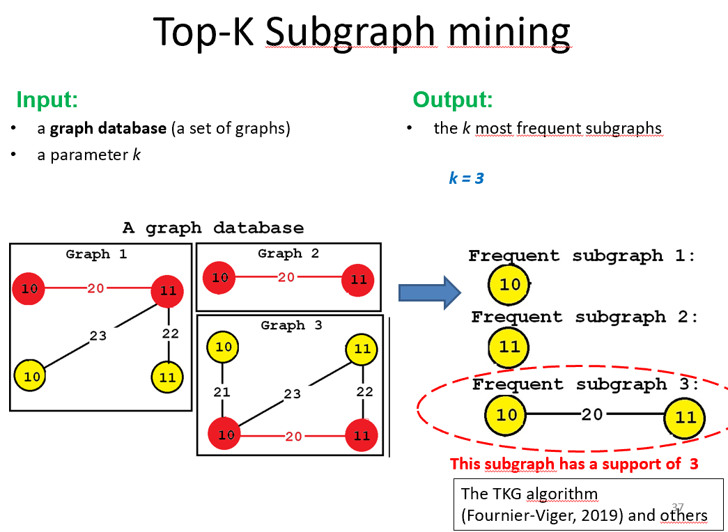
TSPIN: I analyze the complexity of an itemset mining algorithm based on FP-Growth for mining periodic patterns. This also shows how to analyze the complexity of a top-k pattern mining algorithm.
EFIM: I analyze the complexity of an algorithm for high utility itemset mining that does a depth-first search and use a pattern-growth approach.
FHUQI-Miner: I analyze the complexity of a quantiative high utility itemset mining algorithm, which does a depth-first search, and is based on Eclat / HUI-Miner.
CEPB: In this paper, I analyze the complexity of a kind of sequential pattern mining algorithm that uses a pattern-growth approach, and perform a depth-first search.
LHUI-Miner: I analyze the complexity of another algorithm based on HUI-Miner for high utility itemset mining.
Conclusion
That was a blog post to give a rough idea about how to analyze the complexity of pattern mining algorithms. Hope that this blog post is helpful! If you have any comments, you may leave them in the comment section below. Thanks for reading.
Today, I will talk briefly about short papers at academic conferences, and the problems that they create (in my opinion). For those who don’t know, several conferences can reject or accept papers as short or full papers. A short paper means that the paper has fewer pages in the proceedings than the full papers. For instance, someone may submit a 12-page paper to a conference, which may then be accepted as a short paper that must fit in 6 pages.
Why there are short papers? The reason is quite simple. It allows conference organizers to accept more papers for their conference and thus to have more attendees, which means to earn more money through the registration fees (because it is the same price anyway for a short or a full paper). Short papers also allows conferences to accept some papers that are sometimes of low quality (almost rejected in some cases).
Why I dislike short papers? I think they are not a good idea. Let me explain why:
They force authors to remove many important details to try to squeeze their content in a small number of pages. For example, I recently got a paper accepted as short paper, and to make it fit within the page limit, I would have to either remove much of the technical details or remove some experiments. Either way, this will decrease the quality of the paper and the reader will miss some important details.
Not able to address the reviewers’ comments. In many cases, reviewers will give feedback on the paper saying that content must be added such as additional experiments. But if the paper is accepted as a short paper and the paper must be reduced by several pages, authors will be unable to address these comments, and authors may even have to do the opposite and remove experiments and details.
Quality control. Many conferences that accept short papers will not send the revised papers to reviewers again to ensure the quality of the revision. But after cutting let’s say 50% of the content, the quality has a good chance to decrease.
Less chances of having an impact. Short papers are less likely to have an impact or to be cited.
Probably less reproducible. Short papers are generally harder to reproduce because authors may have to left out much details.
The authors have to spend extra time to shorten their paper. To make a paper shorter, it can requires a few days of extra work.
It will likely not be possible to publish the results elsewhere as a full paper. Generally, if someone publish some results or ideas in a short paper, it will likely not be possible to make a full paper on the same idea at another conference (due to the overlap). Someone people may still do this by splitting their ideas into multiple papers but this is not a good practice.
For all these reasons, I dislike short papers, and often withdraw my papers if they are accepted as short papers, and then improve them and submit them to other conferences.
There are also some publishers such as Springer that acknowledge in some way the problem of short papers by mentioning that conferences are not expected to have too many short papers and that it is encouraged to not put a strict limit on the number of pages to avoid reducing the quality of papers.
That is all for today. If you have any comments, you may post them in the comment section below.
I have uploaded a new 38 minutes video to explain rare itemset mining. This video is like a small course, where you can learn about infrequent itemsets, minimal rare itemsets and perfectly rare itemsets and some algorithms : AprioriInverse and AprioriRare.
Today, I will show how to draw a sequence in Latex using the TIKZ package. A sequence is an ordered list of symbols. I often draw sequences for my research paper about sequential pattern mining or episode mining. To draw a sequence, I first import the TIKZ package by adding this line in the section for packages:
\usepackage{tikz}
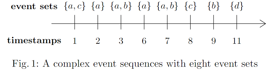
Example 1. To draw a sequence in a figure that looks like this:
I use this code:
\begin{figure}[ht]
\centering
\begin{tikzpicture}
%timeline
\draw (-0.4,0) -- (7,0);
% The labels
\node[] at (-1,0.6) {\textbf{event sets}};
\node[] at (-1,-0.6) {\textbf{timestamps}};
% first element
\draw (0.4,-0.2) -- (0.4,0.3); \node[] at (0.4,0.6) {${a,c}$}; \node[] at (0.4,-0.6) {$1$};
% second element
\draw (1.2,-0.2) -- (1.2,0.3); \node[] at (1.2,0.6) {${a}$}; \node[] at (1.2,-0.6) {$2$};
% third element
\draw (2,-0.2) -- (2,0.3); \node[] at (2,0.6) {${a,b}$}; \node[] at (2,-0.6) {$3$};
% next element
\draw (2.8,-0.2) -- (2.8,0.3); \node[] at (2.8,0.6) {${a}$}; \node[] at (2.8,-0.6) {$6$};
% next element
\draw (3.6,-0.2) -- (3.6,0.3); \node[] at (3.6,0.6) {${a,b}$}; \node[] at (3.6,-0.6) {$7$};
% next element
\draw (4.4,-0.2) -- (4.4,0.3); \node[] at (4.4,0.6) {${c}$}; \node[] at (4.4,-0.6) {$8$};
% next element
\draw (5.2,-0.2) -- (5.2,0.3); \node[] at (5.2,0.6) {${b}$}; \node[] at (5.2,-0.6) {$9$};
% next element
\draw (6,-0.2) -- (6,0.3); \node[] at (6,0.6) {${d}$}; \node[] at (6,-0.6) {$11$};
% The arrow
\draw (6.8,-0.13) -- (7,0);
\draw (6.8,0.13) -- (7,0);
\end{tikzpicture}
\caption{A complex event sequence with eight event sets}
\label{CES}
\end{figure}
You could improve upon this using other options in Tikz to add colors, etc.
Example 2: Another version of that example, with more timestamps:
The Latex code:
\begin{figure}[ht]
  %  \centering
%    \includegraphics[width=0.7\textwidth]{SEQ.pdf}
%\begin{figure}[ht]%
\centering
\begin{tikzpicture}
%timeline
\draw (-0.4,0) -- (10,0);
% The labels
\node[] at (-1,0.6) {\textbf{event sets}};
\node[] at (-1,-0.6) {\textbf{timestamps}};
% first element
\draw (0.4,-0.2) -- (0.4,0.3); \node[] at (0.4,0.6) {$\{c\}$}; \node[] at (0.4,-0.6) {$t_1$};
% second element
\draw (1.2,-0.2) -- (1.2,0.3); \node[] at (1.2,0.6) {$\{a,b\}$}; \node[] at (1.2,-0.6) {$t_2$};
% third element
\draw (2,-0.2) -- (2,0.3); \node[] at (2,0.6) {$\{d\}$};
\node[] at (2,-0.6) {$t_3$};
% next element
\draw (2.8,-0.2) -- (2.8,0.3); \node[] at (2.8,0.6) {}; \node[] at (2.8,-0.6) {$t_4$};
% next element
\draw (3.6,-0.2) -- (3.6,0.3); \node[] at (3.6,0.6) {$\{a\}$}; \node[] at (3.6,-0.6) {$t_5$};
% next element
\draw (4.4,-0.2) -- (4.4,0.3); \node[] at (4.4,0.6) {$\{c\}$}; \node[] at (4.4,-0.6) {$t_6$};
% next element
\draw (5.2,-0.2) -- (5.2,0.3); \node[] at (5.2,0.6) {$\{b\}$}; \node[] at (5.2,-0.6) {$t_7$};
% next element
\draw (6,-0.2) -- (6,0.3); \node[] at (6,0.6) {$\{d\}$}; \node[] at (6,-0.6) {$t_8$};
% next element  9
\draw (7,-0.2) -- (7,0.3); \node[] at (7,0.6) {}; \node[] at (7,-0.6) {$t_9$};
% next element 10
\draw (8,-0.2) -- (8,0.3); \node[] at (8,0.6) {$\{a,b,c\}$}; \node[] at (8,-0.6) {$t_{10}$};
% next element 11
\draw (9,-0.2) -- (9,0.3); \node[] at (9,0.6) {$\{a\}$}; \node[] at (9,-0.6) {$t_{11}$};
% The arrow
\draw (9.8,-0.13) -- (10,0);
\draw (9.8,0.13) -- (10,0);
\end{tikzpicture}
    \caption{A complex event sequence}
    \label{figseq}
\end{figure}
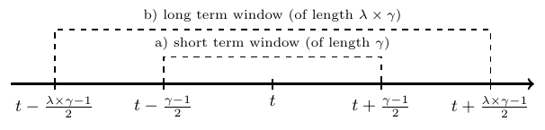
Example 3. Here is a more complicated example. To draw a sequence that looks like this:
I use this code:
\begin{figure}
\centering
%%%%%%%%%%%%%%%%%%%%%%%%%%%%
\begin{tikzpicture}[xscale=8]
\draw[-][draw=black, very thick] (-0.1,0) -- (.5,0);
\draw[->][draw=black, very thick] (.5,0) -- (1.1,0);
%\draw [thick] (0,-.1) node[below]{0} -- (0,0.1);
\draw [thick] (0.25,-.1) node[below]{$t-\frac{\gamma-1}{2}$} -- (0.25,0.1);
\draw [thick] (0,-.1) node[below]{$t-\frac{\lambda\times\gamma-1}{2}$} -- (0,0.1);
%%%%  WINDOW A
\draw [thick, dashed] (0.25,0) -- (0.25,.5) -- (.5,.5) node[above]{
\scriptsize a) short term window (of length $\gamma$)
} -- (0.75,.5) -- (0.75,0) ;
\draw [thick, dashed] (0,0) -- (0,1) -- (.5,1) node[above]{
\scriptsize b) long term window (of length $\lambda \times \gamma $)
} -- (1,1) -- (1,0) ;
\draw [thick] (0.5,-.1) node[below]{$t$} -- (0.5,0.1);
\draw [thick] (0.75,-.1) node[below]{$t+\frac{\gamma-1}{2}$} -- (0.75,0.1);
\draw [thick] (1,-.1) node[below]{$t+\frac{\lambda\times\gamma-1}{2}$} -- (1,0.1);
%\draw [thick] (1,-.1) node[below]{1} -- (1,0.1);
\end{tikzpicture}
%\caption{The windows for calculating the a) short term and b) long term moving average utility  for a timestamp $t$.}

\end{figure}
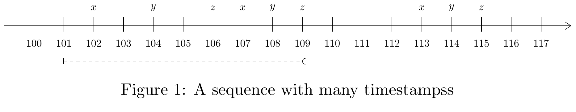
Example 4. And to draw a sequence like this that display some interval:
I use that code:
\begin{figure}[ht]
\centering
	\resizebox{\columnwidth}{!}{
\begin{tikzpicture}
%timeline
\draw (0,0) -- (19,0);
% first element
\draw (1,-0.2) -- (1,0.3);	 \node[] at (1,0.6) { }; 	\node[] at (1,-0.6) {100};
\draw (2,-0.2) -- (2,0.3);	 \node[] at (2,0.6) { }; 	\node[] at (2,-0.6) {101};
% Window 1
\draw[thick] (2,-1.1) -- (2,-1.3); \draw[dashed] (2,-1.2) -- (10,-1.2); \draw(10.1,-1.1) arc (90:270:0.1);
%%%%
\draw (3,-0.2) -- (3,0.3);	 \node[] at (3,0.6) {$x$}; 	\node[] at (3,-0.6) {102};
\draw (4,-0.2) -- (4,0.3);	 \node[] at (4,0.6) { }; 	\node[] at (4,-0.6) {103};
\draw (5,-0.2) -- (5,0.3);	 \node[] at (5,0.6) {$y$}; 	\node[] at (5,-0.6) {104};
\draw (6,-0.2) -- (6,0.3);	 \node[] at (6,0.6) { }; 	\node[] at (6,-0.6) {105};
\draw (7,-0.2) -- (7,0.3);	 \node[] at (7,0.6) {$z$}; 	\node[] at (7,-0.6) {106};
\draw (8,-0.2) -- (8,0.3);	 \node[] at (8,0.6) {$x$}; 	\node[] at (8,-0.6) {107};
\draw (9,-0.2) -- (9,0.3);	 \node[] at (9,0.6) {$y$}; 	\node[] at (9,-0.6) {108};
\draw (10,-0.2) -- (10,0.3);	 \node[] at (10,0.6) {$z$}; 	\node[] at (10,-0.6) {109};
\draw (11,-0.2) -- (11,0.3);	 \node[] at (11,0.6) { }; 	\node[] at (11,-0.6) {110};
\draw (12,-0.2) -- (12,0.3);	 \node[] at (12,0.6) { }; 	\node[] at (12,-0.6) {111};
\draw (13,-0.2) -- (13,0.3);	 \node[] at (13,0.6) { }; 	\node[] at (13,-0.6) {112};
\draw (14,-0.2) -- (14,0.3);	 \node[] at (14,0.6) {$x$}; 	\node[] at (14,-0.6) {113};
\draw (15,-0.2) -- (15,0.3);	 \node[] at (15,0.6) {$y$}; 	\node[] at (15,-0.6) {114};
\draw (16,-0.2) -- (16,0.3);	 \node[] at (16,0.6) {$z$}; 	\node[] at (16,-0.6) {115};
\draw (17,-0.2) -- (17,0.3);	 \node[] at (17,0.6) {}; 	\node[] at (17,-0.6) {116};
\draw (18,-0.2) -- (18,0.3);	 \node[] at (18,0.6) { }; 	\node[] at (18,-0.6) {117};

% The arrow
\draw (18.8,-0.13) -- (19,0);
\draw (18.8,0.13) -- (19,0);
\end{tikzpicture}
}
\caption{A sequence with many timestamps}
\label{CES}
\end{figure}
In this blog post, I will share a simple script to recursively unzip all ZIP files in sub-directories of a directory, and then delete the ZIP files. Such script is useful for example when managing the submissions of papers at academic conferences. The script is based some code on StackOverflow where I have added the function to delete the ZIP files:
FOR /D /r %%F in ("*") DO (
    pushd %CD%
    cd %%F
        FOR %%X in (*.rar *.zip) DO (
            "C:\Program Files\7-zip\7z.exe" x "%%X"
		   del *.zip
        )
    popd
)
This is for Windows. It assumes that you have 7ZIP installed on your computer and that the path to 7ZIP is correct. Save this script into a text file. Rename it to have the .bat extension. Then, double click on the file to run the script. That is all!
This week, I am attending the DASFAA 2022 conference, which is held online from the 11th to the 14th April 2022. In this blog post, I will talk about this event, and will update the blog through the conference.
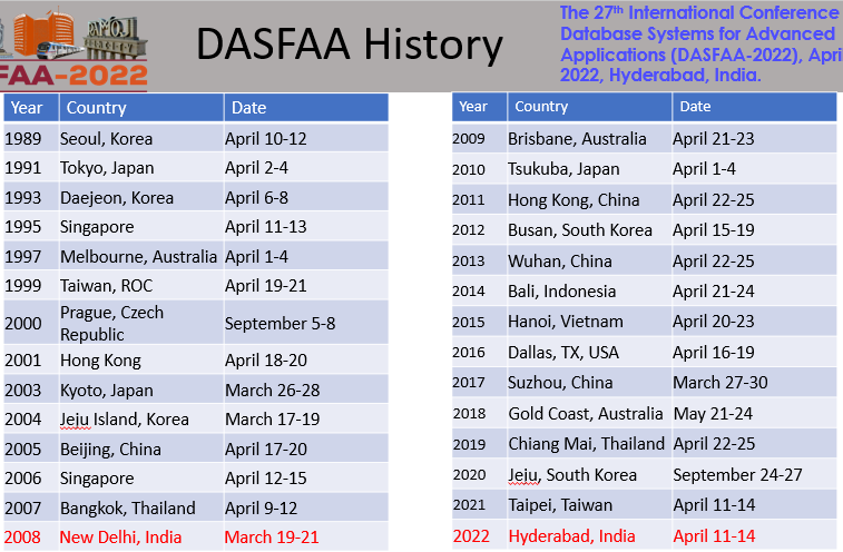
DASFAA 2022 is the 27th International Conference on Database Systems for Advanced Applications. It is a well-established conference on database and related research areas and applications such as data mining and machine learning. This year, it was supposed to be held in India, but due to the pandemic, it was held in online mode. The conference is organized by IIT Hyderabad, India.
The DASFAA Proceedings
The DASFAA conference proceedings are published by Springer in book(s) of the Lecture Notes in Computer Sciences series. This ensures that papers in DASFAA are indexed and have a good visibility.
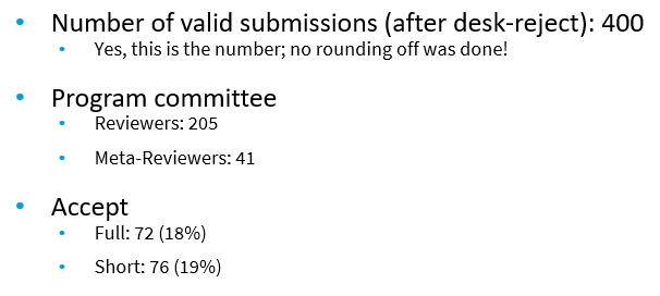
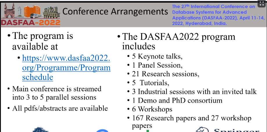
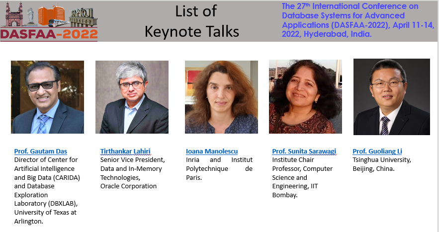
This year the DASFAA program includes 5 keynote talks, 143 research papers, 12 industry presentations, a panel, 11 demos, 5 tutorials and 6 workshops (including the PMDB 2022 workshop on pattern mining and machine learning). It is thus a rather large conference. There was 420 registered attendees.
Acceptance rates
For the main track, there was 400 submissions, and 72 were accepted as full papers ( acceptance rate of 18%) and 76 as short papers (19%).
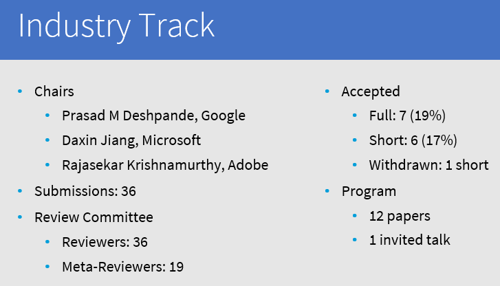
For the industry track, there was 36 submissions, from which there are 7 accepted full papers (19%) and 6 accepted short papers (17%).
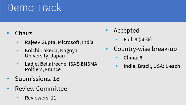
For the demo track, 9 of the 18 submissions were accepted (50%).
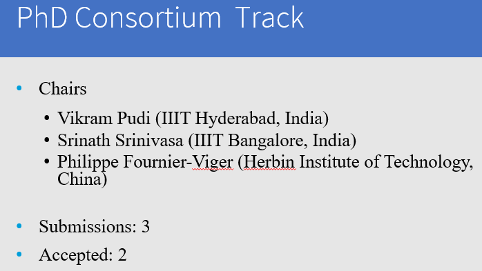
For the PhD track, 2 out of 3 submissions were accepted (66%).
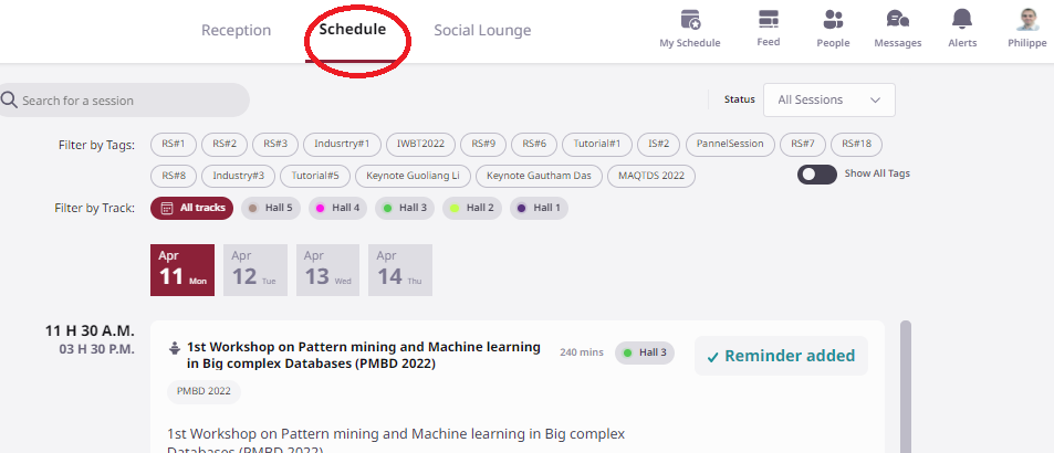
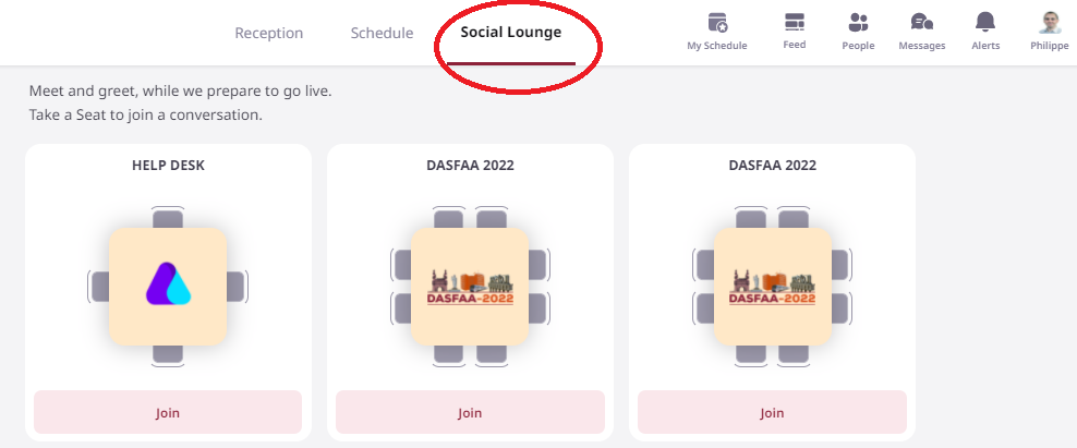
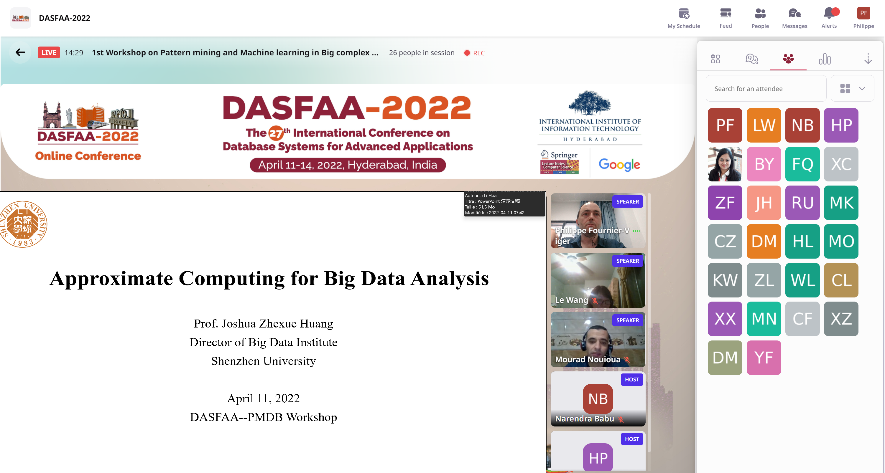
Theonline platform
The conference is held using an online platform called Airmeet. It allows to check the schedule, listen to talks and there are some video chat rooms to socialize with other participants. Here are a few screenshots of that platform. The DASFAA schedule page:
The keynote talk by Prof. Huang, founding director of the big data institute at Shenzhen University was about big data approximate computing. He presented a model called RSP (Random Sample Partition) as an alternative to the popular Hadoop and Spark models. The key idea in RSP is to create distributed data blocks that are random samples of the original data. Then, using these random data blocks, big datasets can be used to train approximate models such as SVM. Using RSP, confidence intervals can be calculated on the errors of approximation. RSP allows to process very large datasets efficiently and provide excellent scalability. In some applications, RSP was shown to have better performance than traditional models such as Hadoop.
Then, there was 6 accepted papers presentations:
9:45
Paper #2 An Algorithm for Mining Fixed-Length High Utility Itemsets (PDF) Le Wang
10:05
Paper #3 A Novel Method to Create Synthetic Samples with Autoencoder Multi-layer Extreme Learning Machine (PDF) Qihang Huang, Yulin He, Shengsheng Xu and Joshua Zhexue Huang
10:25
Paper #4 Pattern Mining: Current Challenges and Opportunities (PDF, video) Philippe Fournier-Viger, Wensheng Gan, Youxi Wu, Mourad Nouioua, Wei Song, Tin Truong and Hai Duong Van
10:45
Paper #7 Why not to Trust Big Data: Identifying Existence of Simpson’s Paradox (PDF) Rahul Sharma, Minakshi Kaushik, Sijo Arakkal Peious, Mahtab Shahin, Ankit Vidhyarthi and Dirk Draheim
11:05
Paper #8 Localized Metric Learning for Large Multi-Class Extremely Imbalanced Face Database (PDF) (best paper award) Seba Susan and Ashu Kaushik
11:25
Paper #9 Top-k dominating queries on incremental datasets (PDF) Jimmy Ming-Tai Wu, Ke Wang and Jerry Chun-Wei Lin
The PMDB workshop has been a success. Thus, we aim to organize it again next year and make it larger.
Day 2 – Conference opening
In the conference opening, the conference was presented. There was a lot of interesting information. As I missed one part of the opening, I would to thank Prof. P.K. Reddy for sharing the slides with me. I will provide a few screenshots of interesting content from the opening below.
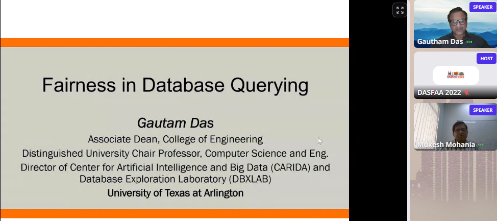
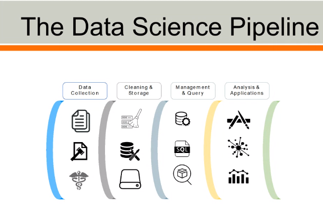
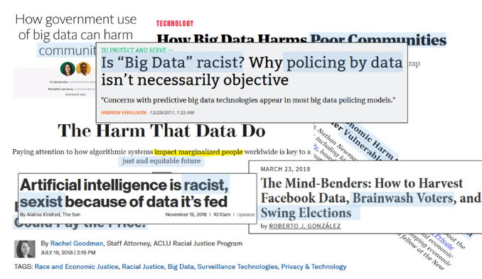
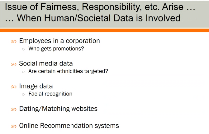
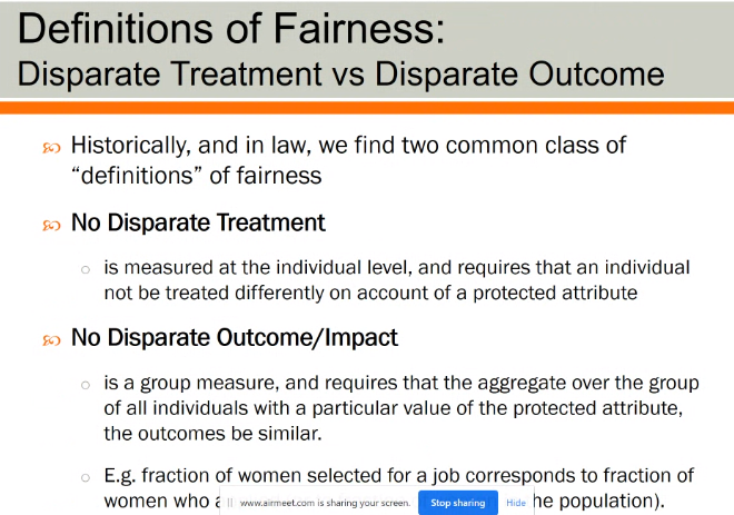
Keynote 1 : Fairness in Database Querying by Gautam Das
The first keynote of the conference was about fairness for database queries. This is an topic that has made the news in recent years with machine learning models that are for example deemed to be racist or unfair to some groups. Here are a few slides:
Research paper presentations
There was numerous paper presentations. I was busy. Thus I will not specifically report on them.
Next year, DASFAA 2023
DASFAA2023 will be in Tianjin, China during April 2023
Conclusion
I have given a brief overview of the DASFAA 2022 conference. Hope that it has been interesting.
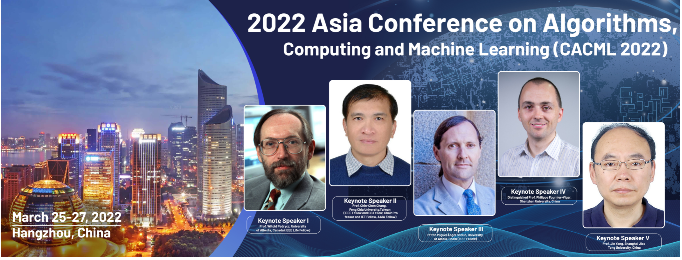
Today, I have attended the CACML 2022 conference (2022 Asia Conference on Algorithms, Computing and Machine Learning), which was held virtually from Hangzhou, China from March 25 to 27.
This is a new conference on a very timely topic of machine learning and computing. The website is : cacml.net. The conference was well organized. The proceedings of the conference are published by IEEE in the IEEE Xplore digital library (indexed by IE, INSTP etc), which provides a good visibility to the paper.
I have been involved in this conference as conference chair, and as keynote speaker.
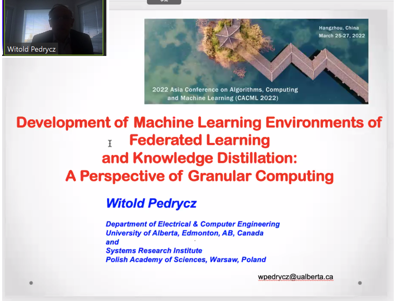
Keynote talk by Prof. Witold Pedrycz
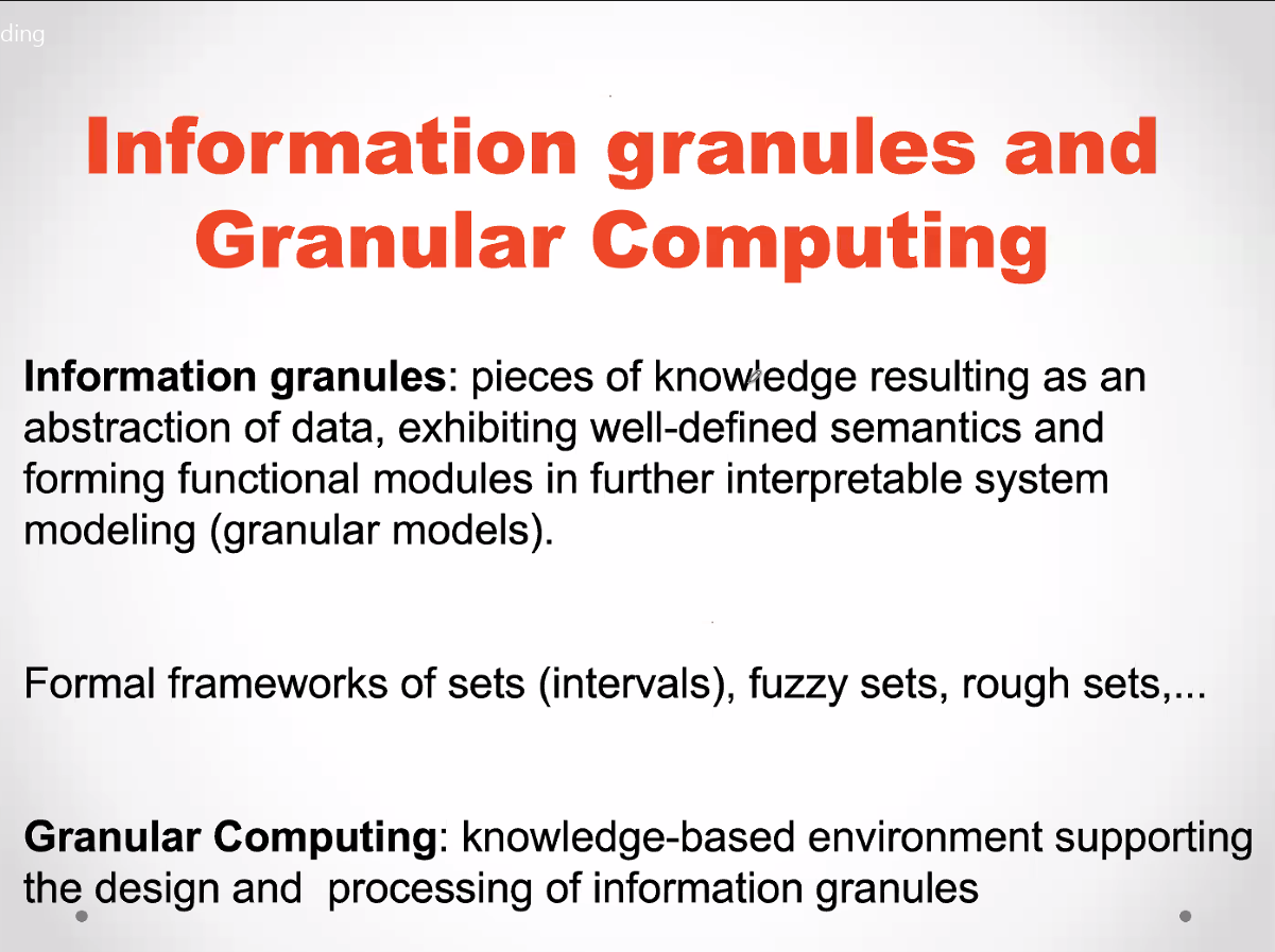
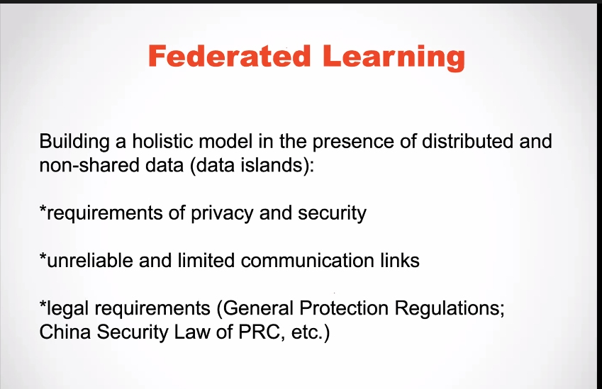
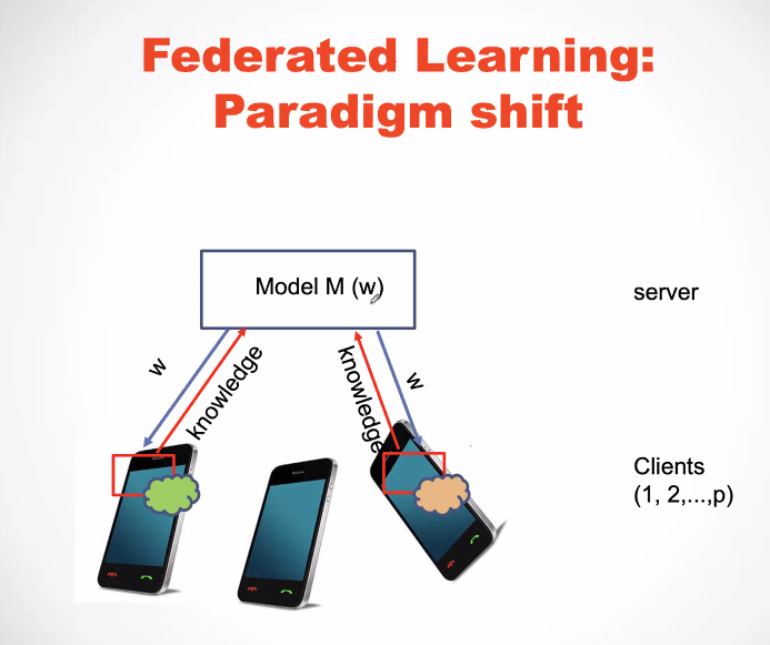
The first talk was by Witold Pedrycz from University of Alberta, Canada, a well-known researcher and editor of the Information Science journal. He talked about machine learning, granular computing and federated learning. Here are a few slides:
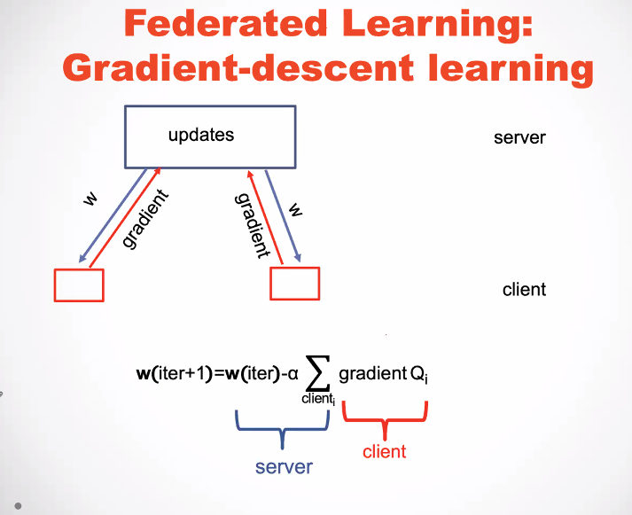
As illustrated in the above slide, in federated learning, each client is the owner of his data. Then, if a server wants to build a machine learning model, the server will interact with the clients to build a model. But the client will not disclose their data to the server. Instead the clients will provide knowledge to the server to help build the model. This is interesting idea to protect the privacy of users. Below, there is another slide that shows how a model is updated in the case of gradient descent with federated learning. Each client returns a gradient to the server rather than sharing the data.
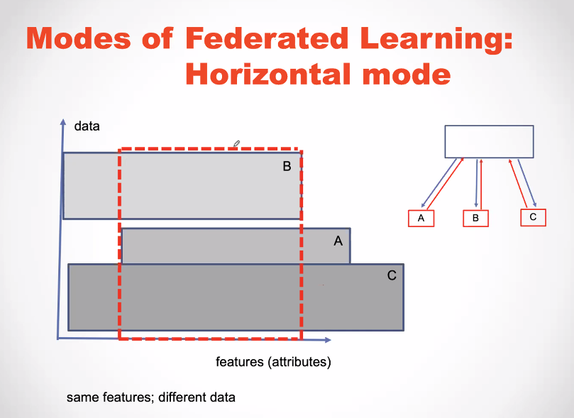
Then, there was more details about how federated learning and granular computing can be used jointly to build rule-based models, and the issue of how to evaluate the quality of the models built using federated learning (since the server does not have access to all the data). I will not report all the details. But it was an interesting talk.
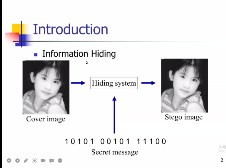
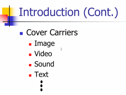
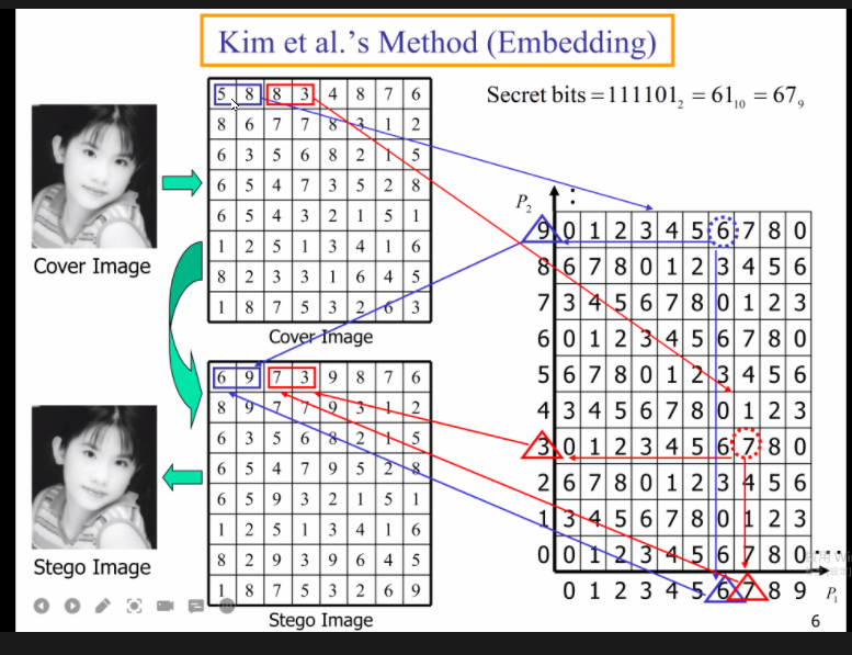
Keynote talk byProf. Chin Chen Chang
The second keynote by Prof. Chin Chen Chang from National Tsing Hua University, Taiwan was about information hiding that is how to hide information, for example, to send a secret message by hiding it inside images.
Keynote talk by Prof. Philippe Fournier-Viger
The third keynote was given by me about “Advances and challenges for the automatic discovery of interesting patterns in data“.
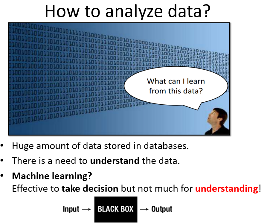
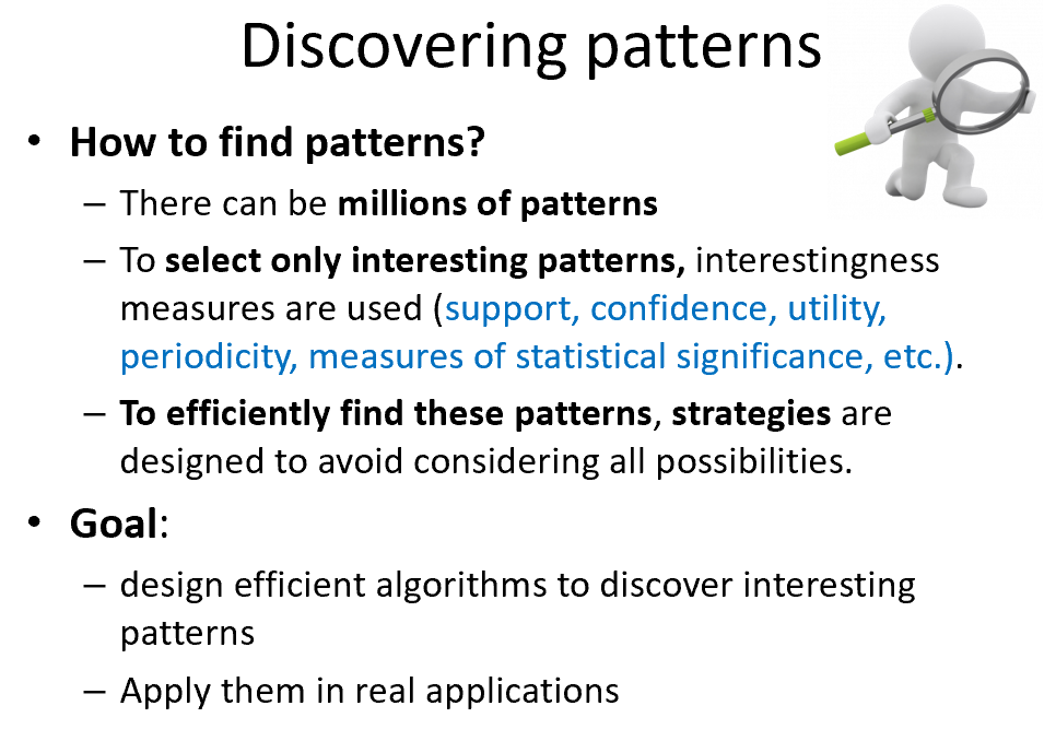
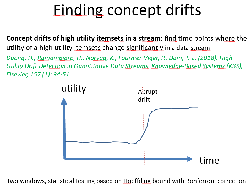
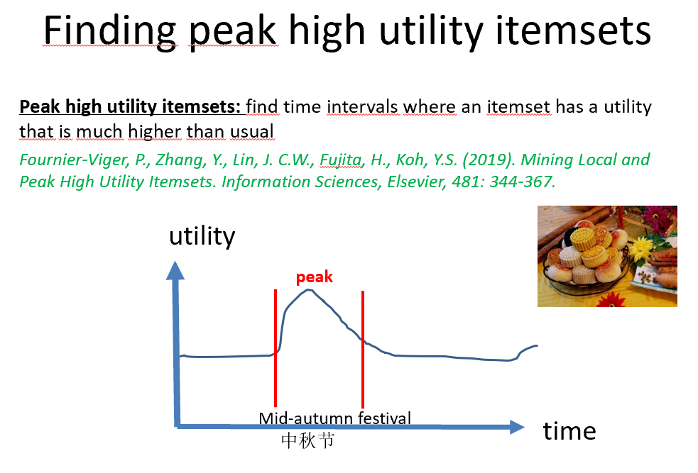
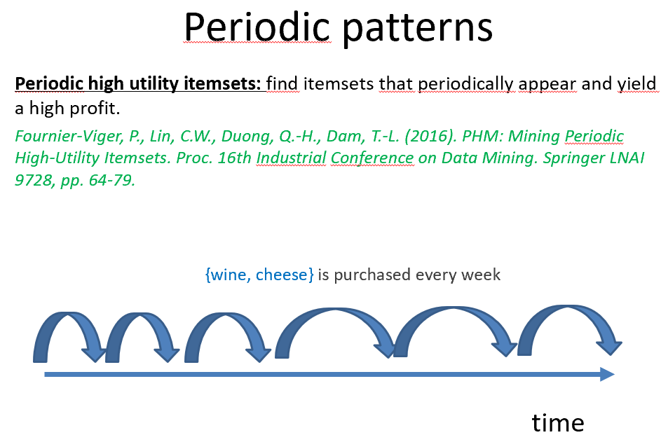
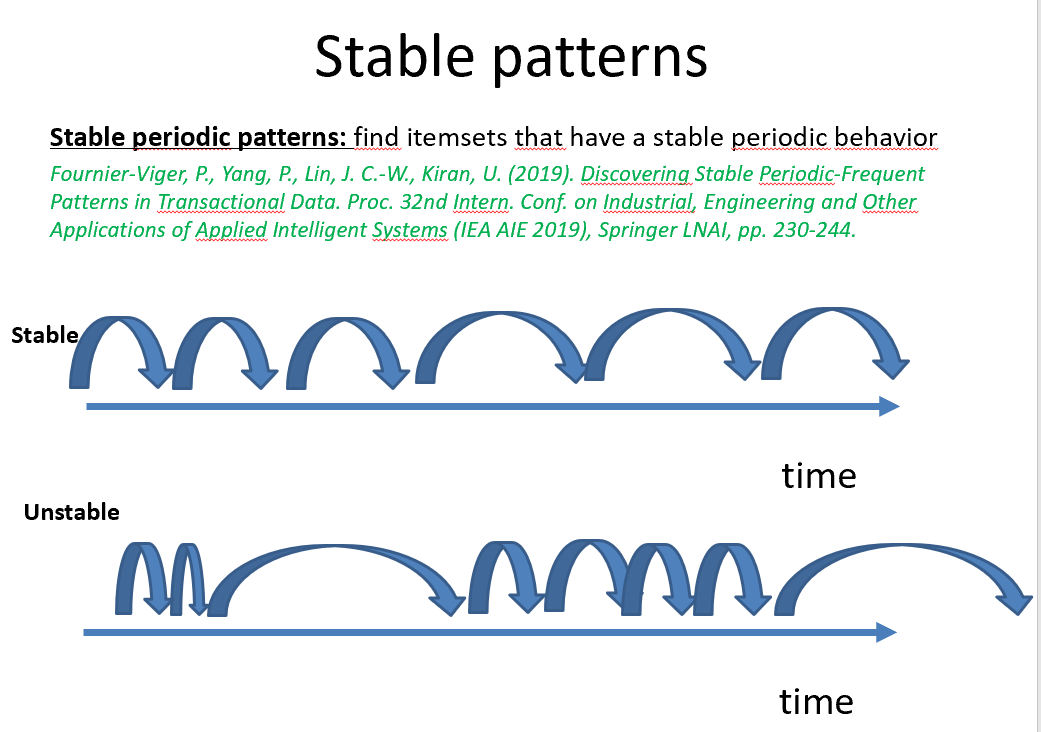
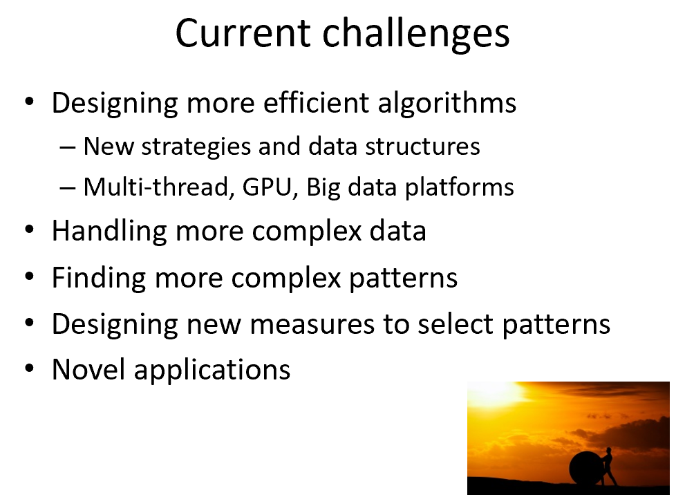
In that talk I briefly reviewed early studies on designing algorithms for identifying frequent patterns that can be used for instance to identify frequent alarms or faults in telecommunication networks. Then, I gave an overview of recent challenges and advances to identify other types of interesting patterns in more complex data. I introduced the concepts of high utility patterns, locally interesting patterns, and periodic patterns. Lastly, the SPMF open-source software will be mentioned and opportunities such as how to combine pattern mining with machine learning.
Keynote talk by Prof. Jie Yang
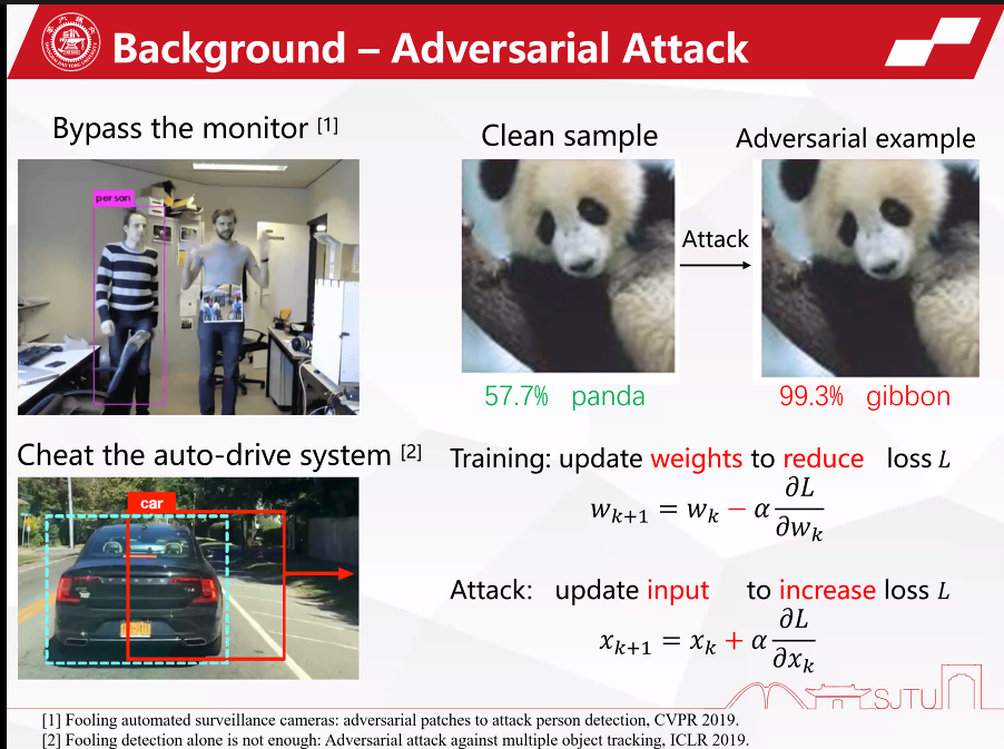
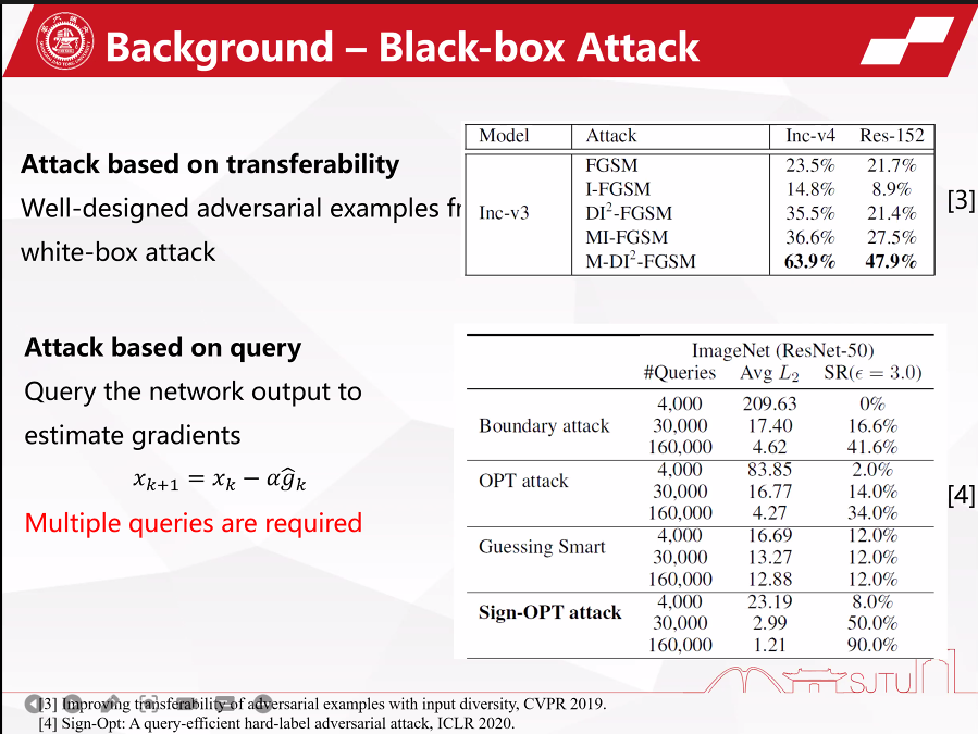
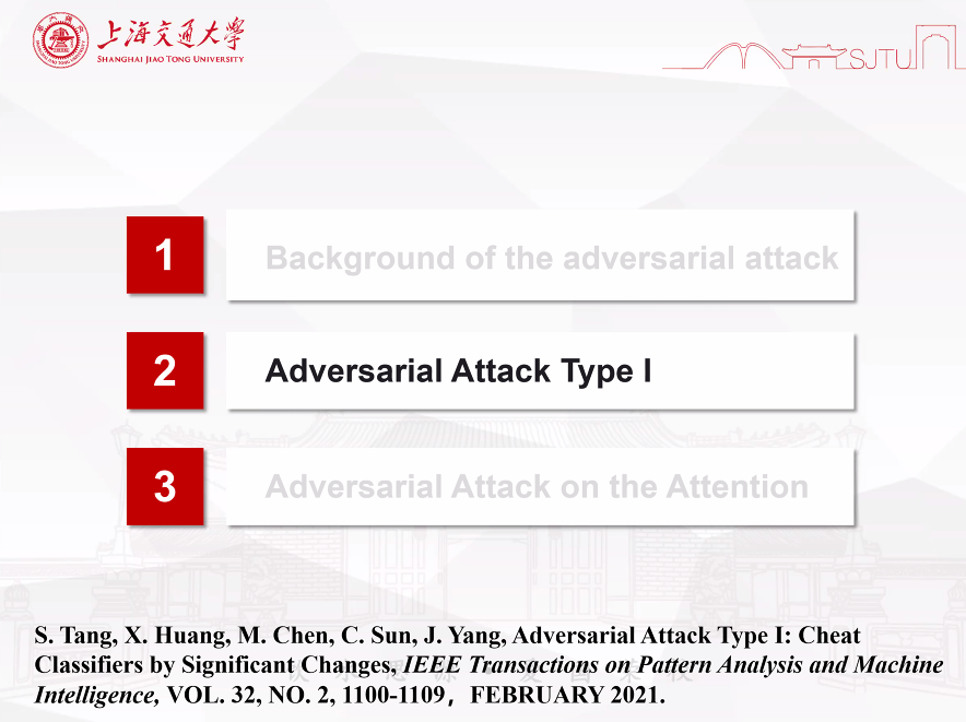
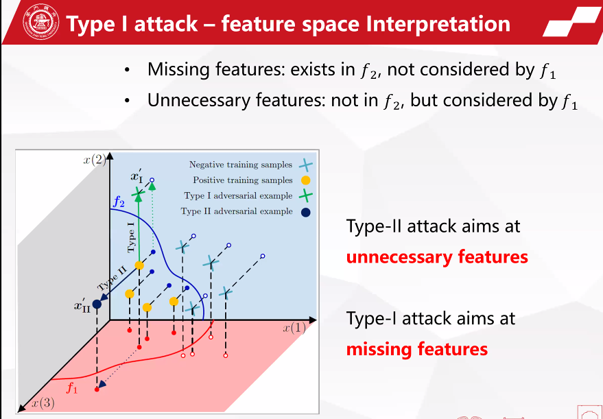
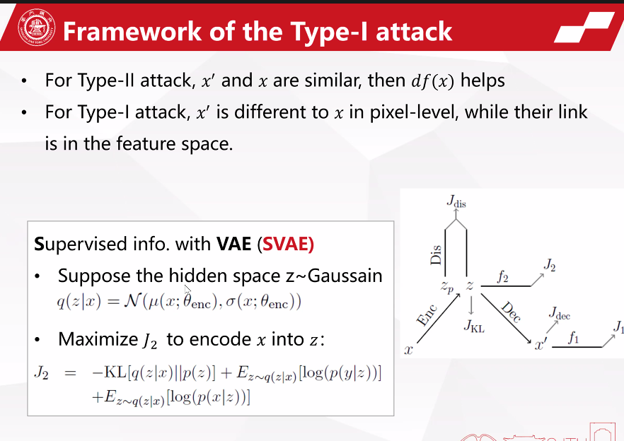
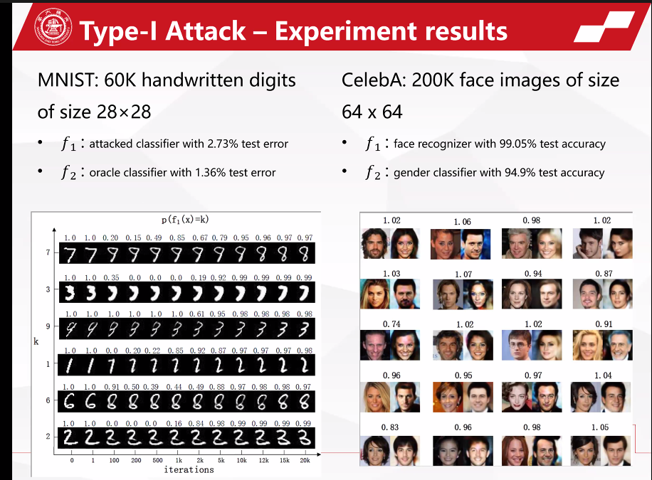
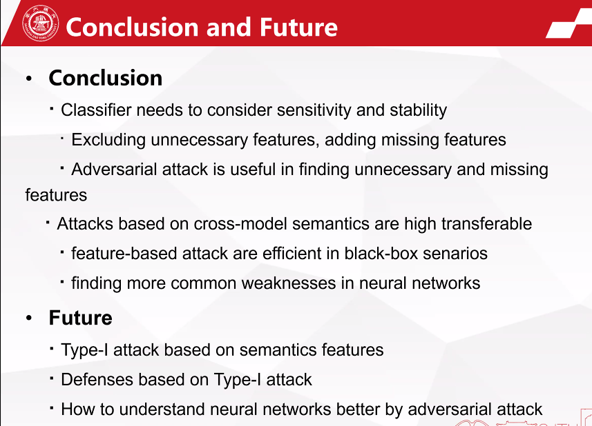
The last keynote talk was by Prof. Jie Yang from Shanghai Jiaotong University about attacks on deep learning models. Here are a few slides:
As shown above, some attacks can be on unnecessary features while other attacks can be about missing features.
There was also some discussion of defense techniques against attacks on neural networks, and attacks on the attention of deep learning models.
Conclusion
This is a short overview of the CACML 2022 conference. It is a medium-size conference (which is understandable since it is a new conference), but there was some good speakers and invited guests. I have enjoyed it, and I would attend again.
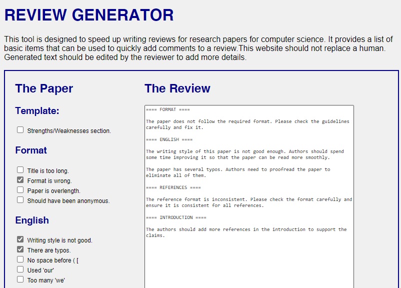
Writing reviews is important but sometimes repetitive and time-consuming. Hence, today I built a tool to help automatize the process of review writing. You can try it at the website below:
This tool let you select some items and this will add predefined sentences to your review. Of course, this tool is not supposed to replace a human and generated reviews should be viewed as draft and edited by hand to add more details.
If you like the tool, you may boomark it and share it. And if you would like more features, please let me know. For example, if you would like that I add more content to the tool, please leave a comment below or send me an email.
** Credit ** That project is a modification of AutoReject (https://autoreject.org/)by Andreas Zeller, which was designed as a joke to automatically reject papers. I have reused the template but modified the text content to turn it into a serious tool. #review#academia#reviewgenerator#reviewprocess#journal#conference
For over two years, I have worked as associate editor-in-chief for a major journal published by Springer. For this job, I have handled around 500 papers from all the steps of the review process. Recently, I have decided to stop this work as it was taking too much of my time and as time is limited in life, I wanted to give priority to other aspects of my life. I was very happy to be associate editor-in-chief for that big journal as this has allowed me to learn many things. I will discuss what I have learned in this blog post. The key things that I have learned are:
Being an editor can be a lot of work. For a big journal, the workload of an editor is quite high. I would spend about one hour every day to try to find reviewers for papers, reading the papers or do other related tasks. One hour may not seem a lot but when you have a research team, a family and other things in your life, it is a lot of time and you have to think about your priorities. With this 1 hour, I could instead do some sport, spend more time with my kid or spend more time on my own research.
Finding reviewers for a paper is not so easy. Authors of research papers often think that reviewers are easy to find. But the truth is that often it is a hard task to find reviewers. The editor has to invite numerous reviewers. Each reviewer has one week or more to accept the invitation. And often the potential reviewers would not answer or decline. Thus, it can happen that it takes over one month to find suitable reviewers for a paper. Generally, if a topic is unpopular, it can be quite hard to find reviewers.
Reviewers are often late. Many authors do not know that it is quite common that reviewers submit their reviews late. Often, it is by a few days, but some reviewers can be late by up to a month in some cases. When a reviewer is late, the journal will automatically send reminders to the reviewer but still some reviewers can receive dozens of reminders and ignore them. In this case, the editor has to step in and find more reviewer(s).
The work of an editor can be repetitive. Although being an editor is interesting and it is also very important for academia, I feel that some work is repetitive such as clicking to find reviewers. Other people will have different opinions but rather than doing such tasks, I would rather spend time working on my own research.
When submitting a paper, if you can enter keywords or select topics from a taxonomy to describe your paper, choose them wisely. It is important to choose keywords that really describe your paper well as this will be used to find reviewers for your paper and can accelerate the review process.
Some reviewers are unethical. As editor, it is important to read carefully what the reviewers write as there are several reviewers that would act unethically such as by asking authors to cite many of their papers to increase their citation count. When i would see this, I would intervene to stop this, of course, but there are always a few reviewers that are trying to do this.
If authors do not do enough effort to revise their paper well (after a round of review), it is not uncommon that a reviewer will change his mind and suggest to reject the paper in the next round. The reviewers are doing their work for free. Some reviewers are very patient and will accept to review the same paper multiple times. But others will not be patient if the author does not make sufficient effort to address issues in the paper. Thus authors should always do their best to solve the problems in their paper.
That was just a short blog post to talk a little bit about the work of an editor and the review process of a journal. I hope it does not sound negative because actually, I have learned many things from this work and I do not regret accepting to do this work.
Hope that this has been interesting. If you have any comments or questions, please leave them in the comment section below!